
Complexity Results for Structure-Based Causality
Proceedings of the Seventeenth International Joint Conference on Artificial Intelligence. Pages 35-41.
© 2001 International Joint Conferences on Artificial Intelligence
Abstract
We analyze the computational complexity of causal relationships in Pearl’s structural models, where we focus on causality between variables, event causality, and probabilistic causality. In particular, we analyze the complexity of the sophisticated notions of weak and actual causality by Halpern and Pearl. In the course of this, we also prove an open conjecture by Halpern and Pearl, and establish other semantic results. To our knowledge, no complexity aspects of causal relationships have been considered so far, and our results shed light on this issue.
- [Balke and Pearl, 1994] A. Balke and J. Pearl. Probabilis- tic evaluation of counterfactual queries. In Proceedings AAAI-94, pages 230-237, 1994.
- [Eiter and Lukasiewicz, 2001] T. Eiter and T. Lukasiewicz. Complexity results for structure-based causality. Techni- cal Report INFSYS RR-1843-01-01, Institut für Informa- tionssysteme, TU Wien, 2001.
- [Galles and Pearl, 1997] D. Galles and J. Pearl. Axioms of causal relevance. Artif. Intell., 97:9-43, 1997.
- [Geffner, 1990] H. Geffner. Causal theories for nonmono- tonic reasoning. In Proc. AAAI-90, pages 524-530, 1990.
- [Geffner, 1992] H. Geffner. Default Reasoning: Causal and Conditional Theories. MIT Press, 1992.
- [Green, 1993] F. Green. On the power of deterministic reduc- tions to Ý # . Math. Syst. Theory, 26(2):215-233, 1993.
- [Halpern and Pearl, 2000] J. Y. Halpern and J. Pearl. Causes and explanations: A structural-model approach. Technical Report R-266, UCLA Cognitive Systems Lab, 2000.
- [Halpern and Pearl, 2001] J. Y. Halpern and J. Pearl. Causes and explanations: A structural-model approach -Part II: Explanation. In Proceedings IJCAI-01, 2001.
- [Halpern, 2000] J. Y. Halpern. Axiomatizing causal reason- ing. J. Artif. Intell. Res., 12:317-337, 2000.
- [Papadimitriou, 1994] C. H. Papadimitriou. Computational Complexity. Addison-Wesley, Reading, MA, 1994.
- [Pearl, 1999] J. Pearl. Reasoning with cause and effect. In Proceedings IJCAI-99, pages 1437-1449, 1999. IJCAI
- [Pearl, 2000] J. Pearl. Causality: Models, Reasoning, and Inference. Cambridge University Press, 2000.
- [Roth, 1996] D. Roth. On the hardness of approximate rea- soning. Artif. Intell., 82(1-2):273-302, 1996. IJCAI
- [Torán, 1991] J. Torán. Complexity classes defined by count- ing quantifiers. J. ACM, 38(3):753-774, 1991.
- [Turner, 1999] H. Turner. A logic of universal causation. Ar- tif. Intell., 113:87-123, 1999.
References were extracted automatically from the PDF and may contain errors.
Full text extracted automatically from the PDF; figures, tables and equations may differ. The PDF is the version of record.
1 Introduction
Representing and reasoning with causal knowledge has received much attention in the recent decade. The existing approaches to causality in the AI literature can be roughly divided into those that have been developed as modal nonmonotonic logics (especially in the context of logic programming) and those that evolved from the area of Bayesian networks.
A representative of the former is Geffner's modal nonmonotonic logic for handling causal knowledge [1990; 1992], which has been inspired by default reasoning from conditional knowledge bases. Other more specialized formalisms play an important role in dealing with causal knowledge about actions and change; see especially the work by Turner [1999] and the references therein for an overview.
A representative of the latter is Pearl's approach to modeling causality by structural equations [Balke and Pearl, 1994; Galles and Pearl, 1997; Pearl, 1999; 2000], which is central to a number of recent research efforts. In particular, the evaluation of deterministic and probabilistic counterfactuals has been explored, which is at the core of problems in fault diagnosis, planning, decision making, and determination of liability [Balke and Pearl, 1994].
In a recent paper, Halpern [2000] gave an axiomatization of reasoning about causal formulas in the structural-model approach, and explored its computational aspects.
It has been shown that the structural-model approach allows a precise modeling of many important causal relationships, which can especially be used in natural language processing [Galles and Pearl, 1997]. In particular, it allows an elegant definition of the important notions of actual causation and explanation [Halpern and Pearl, 2000; 2001].
We give a simple example due to Halpern and Pearl [2000], which illustrates the structural-model approach.
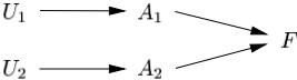
Example 1.1 Suppose that two arsonists lit matches in different parts of a dry forest, and both cause trees to start burning. Assume now that either match by itself suffices to burn down the whole forest. In the structural-model framework, such a scenario may be modeled as follows. We assume two binary background variables ✂ ✄ and ✂ ✆ , which determine the motivation and the state of mind of the two arsonists, where ✂ ✞ has the value 1 iff the arsonist ✠ intends to start a fire. Moreover, we have three binary variables ✡ ✄ , ✡ ✆ , and ✌ , which describe the observable situation, where ✡ ✞ has the value 1 iff the arsonist ✠ drops thematch, and ✌ has the value 1 iff the whole forest burns down. The causal dependencies between these variables are expressed through functions, which say that the value of ✡ ✞ is given by the value of ✂ ✞ , and that ✌ has the value ✎ iff either ✡ ✄ or ✡ ✆ has the value 1. These dependencies can be graphically represented as in Fig. 1.
While the semantic aspects of causal relationships in the structural-model approach have been explored in depth (see especially the work by Pearl [2000]), studies about their computational properties are missing so far. In this paper, we try to fill this gap by giving a precise account of the complexity of deciding causal relationships in structural models.
Note that Halpern's work [2000] is orthogonal to ours, as it focuses on the computational aspects of deciding whether a given causal formula has a causal model, while our work in this paper deals with the complexity of deciding whether a given causal relationship holds in a given causal model.
The main contributions can be summarized as follows:
✏ We analyze the complexity of deciding causal relationships between variables in structural causal models. We consider the notions of causal irrelevance, cause, cause in a context, direct cause, and indirect cause. It turns out that testing these notions has a complexity among ✑ ✒ , ✓ ✔ - ✑ ✒ , and ✖ ✗ . Hardness ✘ holds even in restricted cases.
- ✏ We analyze the complexity of deciding causal relationships between events. We consider the notions of necessary and possible causality, and the sophisticated notions of weak and actual causality by Halpern and Pearl [2000]. In particular, checking the latter is shown to be ✙ ✚ ✆ -complete in general, and ✑ ✒ -complete in the case of binary variables.
- ✏ We prove some semantic results related to the notions of actual and weak causality. More precisely, we prove an open conjecture by Halpern and Pearl [2000], and we give a new characterization of weak causality for the binary case.
- ✏ As a representative for probabilistic causal relationships, we finally analyze the complexity of deciding the notion of probabilistic causal irrelevance, which is shown to be complete for the class C✜ , and thus harder than ✓ ✔ -✑ ✒ . Note that fewC✜ -complete problems, and none in AI, are known.
Our results draw a clear picture of the complexity of structural causality, and give useful insight for exploiting it, e.g., in counterfactual reasoning (see Section 6).
For space reasons, we give only proof sketches of some results. Proofs of all results are given in the extended paper [Eiter and Lukasiewicz, 2001].
2 Preliminaries
We assume a finite set of random variables. Each variable ✢ ✞ may take on values from a finite domain ✣ ✤ ✢ ✞ ✦ . A value for a set of variables ✢ ★ ✩ ✢ ✄ ✬ ✮ ✮ ✮ ✬ ✢ ✯ ✱ is a mapping ✳ ✴ ✢ ✶ ✣ ✤ ✢ ✄ ✦ ✸ ✹ ✹ ✹ ✸ ✣ ✤ ✢ ✯ ✦ such that ✳ ✤ ✢ ✞ ✦ ✾ ✣ ✤ ✢ ✞ ✦ (where the empty mapping ❁ is the unique value for ✢ ★ ❁ ). The domain of ✢ , denoted ✣ ✤ ✢ ✦ , is the set of all values for ✢ . For ❄ ❅ ✢ and ✳ ✾ ✣ ✤ ✢ ✦ , denote by ✳ ❇ ❄ the restriction of ✳ to ❄ . For sets of variables ✢ ✬ ❄ and values ✳ ✾ ✣ ✤ ✢ ✦ and ❊ ✾ ✣ ✤ ❄ ✦ , we use ✳ ❊ to denote the union of ✳ and ❊ . As usual, we often identify singletons ✩ ✢ ✞ ✱ with ✢ ✞ , and their values ✳ with ✳ ✤ ✢ ✞ ✦ .
2.1 Causal and Probabilistic Causal Models
A causal model ❍ is a triple ✤ ✂ ✬ ❑ ✬ ✌ ✦ , where ✂ is a finite set of exogenous variables, ❑ is a finite set of endogenous variables such that ✂ ❖ ❑ ★ ❁ , and ✌ ★ ✩ ✌ a80 ❇ ✢ ✾ ❑ ✱ is a set of functions ✌ a80 ✴ ✣ ✤ ❙ ❚ a80 ✦ ✶ ✣ ✤ ✢ ✦ that assign a value to ✢ for each value of the parents ❙ ❚ a80 ❅ ✂ ✸ ❑ ❳ ✩ ✢ ✱ of ✢ .
We focus here on the principal class of recursive causal models ❍ ★ ✤ ✂ ✬ ❑ ✬ ✌ ✦ (as argued in [Halpern and Pearl, 2000], we do not lose much generality by concentrating on recursive causal models) inwhich a total ordering ❬ on ❑ exists such that ❄ ✾ ❙ ❚ a80 implies ❄ ❬ ✢ , for all ✢ ✬ ❄ ✾ ❑ . In such models, every assignment to the exogenous variables ✂ ★ ❴ determines a unique value ❊ for every set of endogenous variables ❄ ❅ ❑ , denoted ❄ ❜ ✤ ❴ ✦ (or simply ❄ ✤ ❴ ✦ ). In the sequel, ❍ is reserved for denoting a recursive causal model.
For causal models ❍ ★ ✤ ✂ ✬ ❑ ✬ ✌ ✦ , ✢ ❅ ❑ , and ✳ ✾ ✣ ✤ ✢ ✦ , the causal model ❍ a80 ✜ ❡ ★ ✤ ✂ ✬ ❑ ✬ ✌ a80 ✜ ❡ ✦ , where ✌ a80 ✜ ❡ ★ ✩ ✌ ❣ ❇ ❄ ✾ ❑ ❳ ✢ ✱ ✸ ✩ ✌ a80 ✐ ★ ✳ ✤ ✢ ❥ ✦ ❇ ✢ ❥ ✾ ✢ ✱ , is a submodel of ❍ . Intuitively, ✢ is set to ✳ by an "external action". We abbreviate ❍ a80 ✜ ❡ and ✌ a80 ✜ ❡ by ❍ ❡ and ✌ ❡ , respectively. For ❄ ❅ ❑ , we abbreviate ❄ ❜ ♠ ✤ ❴ ✦ by ❄ ❡ ✤ ❴ ✦ .
A probabilistic causal model ✤ ❍ ✬ ❙ ✦ consists of a causal model ❍ ★ ✤ ✂ ✬ ❑ ✬ ✌ ✦ and a probability function ❙ on ✣ ✤ ✂ ✦ .
Example 2.1 In our introductory example, the causal model ❍ ★ ✤ ✂ ✬ ❑ ✬ ✌ ✦ is given by ✂ ★ ✩ ✂ ✄ ✬ ✂ ✆ ✱ , ❑ ★ ✩ ✡ ✄ ✬ ✡ ✆ ✬ ✌ ✱ , and ✌ ★ ✩ ✌ ✉ ✈ ✬ ✌ ✉ ✇ ✬ ✌ ① ✱ , where ✌ ✉ ✈ ★ ✂ ✄ , ✌ ✉ ✇ ★ ✂ ✆ , and ✌ ① ★ ✎ iff ✡ ✄ ★ ✎ or ✡ ✆ ★ ✎ (Fig. 1 shows the parent relationship between the variables). In a probabilistic causal model ✤ ❍ ✬ ❙ ✦ , we may use the uniform distribution ❙ over ✣ ✤ ✂ ✦ .
2.2 Model Representation for Computation
We assume the following representation of causal models ❍ ★ ✤ ✂ ✬ ❑ ✬ ✌ ✦ and probabilistic causal models ✤ ❍ ✬ ❙ ✦ (see the full paper for a discussion of these assumptions):
- ✏ The domain ✣ ✤ ✢ ✦ of each variable ✢ ✾ ✂ ✸ ❑ is explicit, i.e., ✣ ✤ ✢ ✦ ★ ✩ ④ ✄ ✬ ✮ ✮ ✮ ✬ ④ ⑥ ✱ is enumerated.
- ✏ Each function ✌ a80 ✴ ✣ ✤ ❙ ❚ a80 ✦ ✶ ✣ ✤ ✢ ✦ , ✢ ✾ ❑ , is computable in polynomial time.
- ✏ ❙ is given by a pair ✤ ⑧ ✬ ⑨ ✦ , where ⑧ ✴ ✣ ✤ ✂ ✦ ✶ ✩ ❶ ✬ ✎ ✬ ❹ ✬ ✮ ✮ ✮ ✱ is a polynomial-time computable function and ⑨ ❻ ❶ is an integer, such that ❼ ✤ ❴ ✦ ★ ⑧ ✤ ❴ ✦ ❽ ⑨ for every ❴ ✾ ✣ ✤ ✂ ✦ .
The following proposition is immediate.
Proposition 2.2 For every ✢ ✬ ❄ ❅ ❑ and ✳ ✾ ✣ ✤ ✢ ✦ , the values ❄ ✤ ❴ ✦ and ❄ ❡ ✤ ❴ ✦ , given ❴ ✾ ✣ ✤ ✂ ✦ , are computable in polynomial time.
We say ❍ (resp., ✤ ❍ ✬ ❙ ✦ ) is binary, if ❇ ✣ ✤ ✢ ✦ ❇ ★ ❹ for all ✢ ✾ ❑ . Furthermore, ❍ (resp., ✤ ❍ ✬ ❙ ✦ ) is bounded, if ❇ ❙ ❚ a80 ❇ ➀ ➁ holds for each ✢ ✾ ❑ , i.e., ✢ has at most ➁ parents, where ➁ is an arbitrary but fixed constant.
Note that in a bounded model, as for polynomiality, each ✌ a80 is w.l.o.g. given by a table that lists the output values ✌ a80 ✤ ④ ✦ for all ④ ✾ ✣ ✤ ❙ ❚ a80 ✦ (which is similar to a conditional probability table in Bayesian networks).
2.3 Complexity Classes
Complexity classes that we encounter are shown in Fig. 2, where arrows denote containment. ✒ , ✑ ✒ , ✓ ✔ -✑ ✒ , ✙ ✚ ✆ , and ➃ ✚ ✆ are from the Polynomial Hierarchy (PH); ✖ ✗ ★ ✩ ➄ ❖ ➄ ❥ ❇ ➄ ✾ ✑ ✒ ✬ ➄ ❥ ✾ ✓ ✔ - ✑ ✒ ✱ is the "conjunction" of ✑ ✒ and ✓ ✔ - ✑ ✒ . The class C is from the Counting Hierarchy (CH) of complexity classes [Tor´an, 1991]. Informally, C contains all problems which can be expressed as deciding whether a given instance ➅ has at least ⑧ ✤ ❇ ➅ ❇ ✦ many polynomial size "proofs" ➆ ✄ ,. . . , ➆ ➇ ➈ ➉ ➊ ➉ ➋ that ➅ is a Yes-instance, for some function ⑧ , where computing ⑧ ✤ ❇ ➅ ❇ ✦ and checking each proof ➆ ✞ is polynomial. The class C coincides with the famous class ✒ ✒ (probabilistic ✒ ) [Papadimitriou, 1994], which contains the problems decidable by a polynomial-time Turing machine which accepts an input iff the majority of its runs halt in an accepting state.
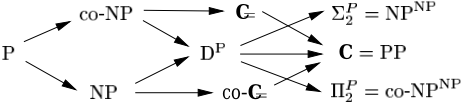
The class C ✜ is a variant of C, where "exactly ⑧ ✤ ❇ ➅ ❇ ✦ " replaces ➍ "at least ⑧ ✤ ❇ ➅ ❇ ✦ ". While this difference seems marginal, C and C✜ have quite different properties [Tor´an, 1991]. Intuitively, C ✜ is an extension of ✓ ✔ - ✑ ✒ , and has many properties of this class. C and C ✜ are contained in PSPACE, and it is believed that they are not contained in PH.
3 Causality between Variables
We first focus on causal relationships between variables due to Galles and Pearl [1997]; see also [Pearl, 1999; 2000].
3.1 Definitions
In the sequel, we assume a causal model ❍ ★ ✤ ✂ ✬ ❑ ✬ ✌ ✦ and sets of variables ✢ ✬ ❄ ✬ ➎ ❅ ❑ with ✢ ✬ ❄ ➏ ★ ❁ . We say
- ✏ ✢ is causally irrelevant to ❄ given ➎ iff for every ➐ ❅ ❑ ❳ ✢ ✸ ❄ ✸ ➎ , ❴ ✾ ✣ ✤ ✂ ✦ , ✳ ✬ ✳ ❥ ✾ ✣ ✤ ✢ ✦ , ➒ ✾ ✣ ✤ ➎ ✦ , and ➓ ✾ ✣ ✤ ➐ ✦ , we have ❄ ❡ ➔ → ✤ ❴ ✦ ★ ❄ ❡ ✐ ➔ → ✤ ❴ ✦ .
- ✏ ✢ is a cause of ❄ iff values ✳ ✬ ✳ ❥ ✾ ✣ ✤ ✢ ✦ and ❴ ✾ ✣ ✤ ✂ ✦ exist such that ❄ ❡ ✤ ❴ ✦ ➏ ★ ❄ ❡ ✐ ✤ ❴ ✦ .
- ✏ ✢ is a cause of ❄ in the context ➎ ★ ➒ iff values ✳ ✬ ✳ ❥ ✾ ✣ ✤ ✢ ✦ and ❴ ✾ ✣ ✤ ✂ ✦ exist with ❄ ❡ ➔ ✤ ❴ ✦ ➏ ★ ❄ ❡ ✐ ➔ ✤ ❴ ✦ .
- ✏ ✢ is a direct cause of ❄ iff values ✳ ✬ ✳ ❥ ✾ ✣ ✤ ✢ ✦ , ❴ ✾ ✣ ✤ ✂ ✦ , and ➒ ✾ ✣ ✤ ❑ ❳ ✢ ✸ ❄ ✦ exist with ❄ ❡ ➔ ✤ ❴ ✦ ➏ ★ ❄ ❡ ✐ ➔ ✤ ❴ ✦ .
- ✏ ✢ is an indirect cause of ❄ iff ✢ is a cause of ❄ and ✢ is not a direct cause of ❄ .
We give some examples of such causal relationships. For a more detailed discussion of these concepts see [Galles and Pearl, 1997] and [Pearl, 1999; 2000].
Example 3.1 In our running example, ✡ ✄ is not causally irrelevant to ✌ . For instance, if we set ✡ ✆ ✾ ❑ ❳ ✩ ✡ ✄ ✬ ✌ ✱ to 0 and ✡ ✄ to 0 and 1, then ✌ has the values 0 and 1, respectively. Informally, the actions of arsonist 1 are not causally irrelevant to the state of the forest. In fact, ✡ ✄ is a cause of ✌ , but not a cause of ✌ in the context ✡ ✆ ★ ✎ . Informally, the actions of arsonist 1 are in general a cause of the state of the forest, but not when arsonist 2 starts a fire. Finally, it is easy to verify that ✡ ✄ is in fact a direct cause of ✌ .
3.2 Results
Our complexity results for checking the above notions of causality are summarized in Table 1. It is important to point out that for all these causal relationships, hardness holds even if ❍ is binary and bounded, and ✢ is a singleton.
| ✢ is causally irrelevant to ❄ given ➎ | ✓ ✔ -✑ ✒ -complete |
| ✢ is a cause of ❄ | ✑ ✒ -complete |
| ✢ is a cause of ❄ in the context ➎ ★ ➒ | ✑ ✒ -complete |
| ✢ is a direct cause of ❄ ✢ is an indirect cause of | ✑ ✒ -complete ✗ |
| ❄ | ✖ -complete |
Our first result shows that deciding causal irrelevance is ✓ ✔ -✑ ✒ -complete. We sketch the main ideas of its proof.
Theorem 3.2 Given ❍ ★ ✤ ✂ ✬ ❑ ✬ ✌ ✦ and ✢ ✬ ❄ ✬ ➎ ❅ ❑ with ✢ ✬ ❄ ➏ ★ ❁ , deciding whether ✢ is causally irrelevant to ❄ given ➎ is ✓ ✔ -✑ ✒ -complete. Hardness holds even if (1) ❍ is binary and bounded, (2) ➎ is empty, (3) ✢ is a singleton, and (4a) ❄ is a singleton or (4b) ❑ ★ ✢ ✸ ❄ ✸ ➎ .
Proof (sketch). The problem is in ✓ ✔ - ✑ ✒ , as ➐ ❅ ❑ ❳ ✢ ✸ ❄ ✸ ➎ and values ❴ ✾ ✣ ✤ ✂ ✦ , ✳ ✬ ✳ ❥ ✾ ✣ ✤ ✢ ✦ , ➒ ✾ ✣ ✤ ➎ ✦ , and ➓ ✾ ✣ ✤ ➐ ✦ such that ❄ ❡ ➔ → ✤ ❴ ✦ ➏ ★ ❄ ❡ ✐ ➔ → ✤ ❴ ✦ can be guessed and verified in polynomial time (see Proposition 2.2).
We show ✓ ✔ - ✑ ✒ -hardness by a polynomial transformation from the ✓ ✔ -✑ ✒ -complete problem of deciding whether a given propositional formula in 3DNF ➛ ★ ➛ ✄ ➜ ✹ ✹ ✹ ➜ ➛ ⑥ on the atoms ✡ ✄ ✬ ✮ ✮ ✮ ✬ ✡ ✯ , where w.l.o.g. ➁ ➝ ❹ and ➞ ➝ ✎ , is a tautology.
We now construct ❍ ★ ✤ ✂ ✬ ❑ ✬ ✌ ✦ and ✢ ✬ ❄ ✬ ➎ ❅ ❑ such that ✢ is causally irrelevant to ❄ given ➎ iff ➛ is a tautology. We define ✢ ★ ✩ ✡ ✱ , ❄ ★ ✩ ➟ ✱ , and ➎ ★ ❁ . Moreover, ✂ ★ ✩ ✡ ✄ ✬ ✮ ✮ ✮ ✬ ✡ ✯ ✱ and ❑ ★ ✢ ✸ ❄ ✸ ✩ ✣ ✄ ✬ ✮ ✮ ✮ ✬ ✣ ⑥ ➡ ✄ ✱ . Let all variables have the domain ✩ ❶ ✬ ✎ ✱ , where 0 and 1 are identified with the truth values ➢ ➤ ➥ ➦ ➧ and ➨ ➩ ➫ ➧ , respectively. The values ❶ and ✎ of ✢ are denoted by ✳ ➭ and ✳ ✄ , respectively. The functions ✌ ➲ for ➳ ✾ ❑ are as follows:
- ✏ ✌ ✉ ★ ✎ and ✌ ➵ ✈ ★ ✡ ➜ ➛ ✄ ,
- ✏ ✌ ➵ ➸ ★ ✣ ✞ ➡ ✄ ➜ ➛ ✞ for all ✠ ✾ ✩ ❹ ✬ ✮ ✮ ✮ ✬ ➁ ➻ ✎ ✱ ,
- ✏ ✌ ➼ ★ ✣ ⑥ ➡ ✄ ➜ ➛ ⑥ .
It can now be shown that ✢ is causally irrelevant to ❄ given ➎ iff ➛ is a tautology. Informally, under any ❴ ✾ ✣ ✤ ✂ ✦ , if ✢ is set to ✳ ✄ , then ❄ becomes 1. Whereas, if ✢ is set to ✳ ➭ , then ❄ is the truth value of ➛ under ❴ . That is, setting ✢ to ✳ ➭ and ✳ ✄ yields the same value of ❄ under any ❴ ✾ ✣ ✤ ✂ ✦ iff ➛ is a tautology. Notice that assignments to some nonempty ➐ ❅ ✣ ✄ ✬ ✮ ✮ ✮ ✬ ✣ ⑥ ➡ ✄ always yield the same value of ❄ .
Note that (1)-(3) and (4a) are satisfied. The proof of hardness in the case where (1)-(3) and (4b) holds is similar. ➽
The following result shows that deciding causes and causes in a context is NP-complete. Here, NP-hardness can be shown by a reduction from the NP-complete problem of deciding whether a propositional formula is not a tautology.
Theorem 3.3 Given ❍ ★ ✤ ✂ ✬ ❑ ✬ ✌ ✦ and ✢ ✬ ❄ ❅ ❑ (resp., ✢ ✬ ❄ ✬ ➎ ❅ ❑ and ➒ ✾ ✣ ✤ ➎ ✦ ) with ✢ ✬ ❄ ➏ ★ ❁ , deciding whether ✢ is a cause of ❄ (resp., ✢ is a cause of ❄ in the context ➎ ★ ➒ ) is ✑ ✒ -complete. Hardness holds even if (1) ❍ is binary and bounded, and (2) ✢ and ❄ are singletons.
4 Event Causality
We now focus on causality between events. In particular, we consider causal relationships between events due to Galles and Pearl [1997]; see also [Pearl, 1999; 2000], and the notions of weak and actual causality by Halpern and Pearl [2000], which are inspired by Pearl's causal beams [2000].
4.1 Definitions
A primitive event is an expression of the form ❄ ★ ❊ , where ❄ is a variable and ❊ is a value for ❄ . The set of events is the closure of the set of primitive events under the Boolean operations ➾ ➚ and ➪ (that is, every primitive event is an event, and if ➛ and ➶ are events, then also ➚ ➛ and ➛ ➪ ➶ ).
The truth of an event ➛ in a causal model ❍ ★ ✤ ✂ ✬ ❑ ✬ ✌ ✦ under ❴ ✾ ✣ ✤ ✂ ✦ , denoted ✤ ❍ ✬ ❴ ✦ ❇ ★ ➛ , is inductively given by:
- ✏ ✤ ❍ ✬ ❴ ✦ ❇ ★ ❄ ★ ❊ iff ❄ ❜ ✤ ❴ ✦ ★ ❊ ,
- ✏ ✤ ❍ ✬ ❴ ✦ ❇ ★ ➚ ➛ iff ✤ ❍ ✬ ❴ ✦ ❇ ★ ➛ does not hold,
- ✏ ✤ ❍ ✬ ❴ ✦ ❇ ★ ➛ ➪ ➶ iff ✤ ❍ ✬ ❴ ✦ ❇ ★ ➛ and ✤ ❍ ✬ ❴ ✦ ❇ ★ ➶ .
We write ➛ ✤ ❴ ✦ to abbreviate ✤ ❍ ✬ ❴ ✦ ❇ ★ ➛ . For ✢ ❅ ❑ and ✳ ✾ ✣ ✤ ✢ ✦ , we write ➛ ❡ ✤ ❴ ✦ to abbreviate ✤ ❍ ❡ ✬ ❴ ✦ ❇ ★ ➛ . For ✢ ★ ✩ ✢ ✄ ✬ ✮ ✮ ✮ ✬ ✢ ⑥ ✱ ❅ ❑ with ➁ ➝ ✎ and ✳ ✞ ✾ ✣ ✤ ✢ ✞ ✦ , we use ✢ ★ ✳ ✄ ✹ ✹ ✹ ✳ ⑥ to abbreviate ✢ ✄ ★ ✳ ✄ ➪ ✮ ✮ ✮ ➪ ✢ ⑥ ★ ✳ ⑥ .
The following proposition is immediate.
Proposition 4.1 Let ✢ ❅ ❑ and ✳ ✾ ✣ ✤ ✢ ✦ . Given ❴ ✾ ✣ ✤ ✂ ✦ and an event ➛ , deciding whether ➛ ✤ ❴ ✦ and ➛ ❡ ✤ ❴ ✦ (given ✳ ) hold can be done in polynomial time.
We are now ready to define causal relationships between events. We first define the notions of necessary and possible causality (which are slightly more general than in [Galles and Pearl, 1997]). Let ❍ ★ ✤ ✂ ✬ ❑ ✬ ✌ ✦ be a causal model. Let ✢ ❅ ❑ and ✳ ✾ ✣ ✤ ✢ ✦ . Let ➛ be an event. We say
- ✏ ✢ ★ ✳ always causes ➛ iff (i) ➛ ❡ ✤ ❴ ✦ for all ❴ ✾ ✣ ✤ ✂ ✦ , and (ii) some ✳ ❥ ✾ ✣ ✤ ✢ ✦ , ❴ ❥ ✾ ✣ ✤ ✂ ✦ exist with ✳ ❥ ➏ ★ ✳ and ➚ ➛ ❡ ✐ ✤ ❴ ❥ ✦ .
- ✏ ✢ ★ ✳ may have caused ➛ iff (i) ✢ ★ ✳ and ➛ are observed (which implies that ✢ ✤ ❴ ✦ ★ ✳ and ➛ ✤ ❴ ✦ for some ❴ ✾ ✣ ✤ ✂ ✦ ) and (ii) some ✳ ❥ ✾ ✣ ✤ ✢ ✦ and ❴ ✾ ✣ ✤ ✂ ✦ exist such that ✳ ❥ ➏ ★ ✳ , ✢ ✤ ❴ ✦ ★ ✳ , ➛ ✤ ❴ ✦ , and ➚ ➛ ❡ ✐ ✤ ❴ ✦ .
We next define weak and actual causality. We say ✢ ★ ✳ is
a weak cause of ➛ under ❴ iff the following conditions hold: AC1. ✢ ✤ ❴ ✦ ★ ✳ and ➛ ✤ ❴ ✦ .
AC2. Some set of variables ➐ ❅ ❑ ❳ ✢ and some values ✳ ✾ ✣ ✤ ✢ ✦ and ➓ ✾ ✣ ✤ ➐ ✦ exist such that:
- (a) ➚ ➛ ❡ → ✤ ❴ ✦ ,
We say ✢ ★ ✳ is an actual cause of ➛ under ❴ iff additionally the following condition is satisfied:
AC3. ✢ is minimal. That is, no proper subset of ✢ satisfies both AC1 and AC2.
We give some illustrative examples.
Example 4.2 In our running example, each event among ✡ ✄ ★ ✎ , ✡ ✆ ★ ✎ , and ✡ ✄ ★ ✎ ➪ ✡ ✆ ★ ✎ always causes ✌ ★ ✎ . For instance, let us show that ✡ ✄ ★ ✎ always causes ✌ ★ ✎ : (i) if ✡ ✄ is set to 1, then ✌ has the value 1 under every ❴ ✾ ✣ ✤ ✂ ✦ , and (ii) if ✂ ✆ is set to 0, and ✡ ✄ to 0, then ✌ has the value 0. Informally, at least one arsonist starting a fire always has the effect that the whole forest burns down.
Consider now the background context ❴ ★ ✤ ✎ ✬ ✎ ✦ in which both arsonists intend to start a fire. Then, each among ✡ ✄ ★ ✎ , ✡ ✆ ★ ✎ , and ✡ ✄ ★ ✎ ➪ ✡ ✆ ★ ✎ is a weak cause of ✌ ★ ✎ . For instance, let us show that ✡ ✄ ★ ✎ is a weak cause of ✌ ★ ✎ : (AC1) both ✡ ✄ and ✌ have the value 1 under ❴ , (AC2 (a)) if both ✡ ✄ and ✡ ✆ are set to 0, then ✌ has the value 0, and (AC2 (b)) if ✡ ✄ is set to 1 and ✡ ✆ to 0, then ✌ has the value 1. In fact, ✡ ✄ ★ ✎ and ✡ ✆ ★ ✎ are actual causes of ✌ ★ ✎ , while ✡ ✄ ★ ✎ ➪ ✡ ✆ ★ ✎ is not an actual cause of ✌ ★ ✎ .
4.2 Results
Our complexity results for the above causal relationships between events are summarized in Table 2. We distinguish between the general and the binary case, in which we assume a syntactic restriction to binary causal models. We remark that for all these causal relationships between events, hardness holds even if ❍ is bounded and ✢ is a singleton.
| Problem | general case | binary case |
|---|---|---|
| ✢ ★ ✳ always causes ➛ ✢ ★ ✳ may cause ➛ ✢ ★ ✳ is a weak cause of ➛ ✢ ★ ✳ is an actual cause of | ✖ ✗ -complete ✑ ✒ -complete ✙ ✚ ✆ -complete ➛ ✙ ✚ ✆ -complete | ✖ ✗ -complete ✑ ✒ -complete ✑ ✒ -complete ✑ ✒ -complete |
The following theorem shows that deciding weak causality is ✙ ✚ ✆ -complete in the general case. We sketch the main ideas behind the technically quite involved proof of this result.
Theorem 4.3 Given ❍ ★ ✤ ✂ ✬ ❑ ✬ ✌ ✦ , ✢ ❅ ❑ , ✳ ✾ ✣ ✤ ✢ ✦ , ❴ ✾ ✣ ✤ ✂ ✦ , and an event ➛ , deciding whether ✢ ★ ✳ is a weak cause of ➛ under ❴ is ✙ ✚ ✆ -complete. Hardness holds even if ✢ is a singleton, and either ❍ is bounded or ➛ is primitive.
Proof (sketch). As for membership in ✙ ✚ ✆ , recall that ✢ ★ ✳ is a weak cause of ➛ under ❴ iff AC1 and AC2 hold. By Proposition 4.1, verifying ✢ ✤ ❴ ✦ ★ ✳ and ➛ ✤ ❴ ✦ is polynomial. Moreover, some ➐ , ✳ , and ➓ as in AC2 can be guessed and verified with an NP-oracle (needed for (b)) in polynomial time. In summary, checking AC1 and AC2 is in ✙ ✚ ✆ .
✙ ✚ ✆ -hardness is shown by a reduction from evaluating a quantifiedBoolean formula ➬ ★ ➮ ✡ ➱ ➟ ✃ , where ✃ is a propositional formula on the variables ✡ ★ ✩ ✡ ✄ ✬ ✮ ✮ ✮ ✬ ✡ ❐ ✱ and ➟ ★ ✩ ➟ ✄ ✬ ✮ ✮ ✮ ✬ ➟ ✯ ✱ . We now define ❍ , etc. as stated such that ✢ ★ ✳ is a weak cause of ➛ under ❴ iff ➬ is true (deciding this is ✙ ✚ ✆ -complete [Papadimitriou, 1994]).
We define ✢ ★ ✩ ❒ ✱ and ❄ ★ ✩ ❮ ✱ . The exogenous and endogenous variables are ✂ ★ ✩ ❰ ✱ and ❑ ★ ✢ ✸ ❄ ✸ ✩ a207 ✱ ✸ ✡ ✸ ➟ , respectively. Define ✣ ✤ ➳ ✦ ★ ✩ ❶ ✬ ✎ ✬ ❹ ✱ for all ➳ ✾ ➟ , and ✣ ✤ ➳ ✦ ★ ✩ ❶ ✬ ✎ ✱ for all ➳ ✾ ✂ ✸ ❑ ❳ ➟ . We define
where ✃ ❥ is obtained from ✃ by replacing each ➳ ✾ ✡ ✸ ➟ by "➳ ★ ✎ ". The functions ✌ ➲ with ➳ ✾ ❑ are defined by:
- ✏ ✌ ➲ ★ ❶ for all ➳ ✾ ✢ ✸ ✩ a207 ✱ ✸ ✡ ,
- ✏ ✌ ➲ ★ ❒ a212 a207 for all ➳ ✾ ➟ , and ✌ a213 ★ ✎ iff ➛ ❥ is true.
Let ❴ ✾ ✣ ✤ ✂ ✦ and ✳ ★ ❶ . Let ➛ be ❄ ★ ✎ . It can now be shown that ✢ ★ ✳ is a weak cause of ➛ under ❴ iff ➬ is true. More precisely, AC1 is trivially satisfied, and AC2 holds iff ➬ is true. Roughly speaking, the existential and universal quantification over ✡ and ➟ in ➬ is reflected by the variables in ➐ and ❑ ❳ ✤ ✢ ✸ ➐ ✦ , respectively. We then especially have to ensure that (i) ➟ ❖ ➐ ★ ❁ and (ii) no truth assignment to the variables in ➟ is ignored. In detail, tomake ➛ false inAC2 (a), a207 must be set to ✎ and all ➳ ✾ ➟ must have the value ❹ . Whereas, to make ➛ true in AC2 (b), all ➳ ✾ ➟ must a215 have a value from ✩ ❶ ✬ ✎ ✱ . This already ensures (i). Since ❒ is set to 0 in AC2 (b), and ✌ ➲ ★ ❒ a212 a207 for all ➳ ✾ ➟ , each variable in ➟ has the value ✎ in AC2 (b). As every ➳ ✾ ➟ has the value 0 in ❍ , this then ensures (ii).
Note that ✢ is a singleton and that ➛ is primitive. To show ✙ ✚ ✆ -hardness for a singleton ✢ and bounded ❍ , define ❍ ❥ ★ ✤ ✂ ✬ ❑ ❳ ✩ ❮ ✱ ✬ ✌ ❳ ✩ ✌ a213 ✱ ✦ . Then, ✢ ★ ✳ is a weak cause of ➛ ❥ under ❴ iff ➬ evaluates to true. ➽
The just sketched proof of ✙ ✚ ✆ -hardness makes use of nonbinary causal models. Thus, we may ask whether deciding weak causality in the binary case has a lower complexity.
In fact, the following semantic result shows that in the binary case, AC2 can be expressed in a different way.
Theorem 4.4 Let ❍ ★ ✤ ✂ ✬ ❑ ✬ ✌ ✦ be binary. Let ✢ ❅ ❑ and ✳ ✾ ✣ ✤ ✢ ✦ . Let ➛ be an event. Then, ✢ ★ ✳ is a weak cause of ➛ under ❴ ✾ ✣ ✤ ✂ ✦ iff AC1 holds, and (AC2') some ➐ ❅ ❑ ❳ ✢ , ✳ ✾ ✣ ✤ ✢ ✦ , and ➓ ✾ ✣ ✤ ➐ ✦ exist such that (a) ➚ ➛ ❡ → ✤ ❴ ✦ , (b) ➛ ❡ → ✤ ❴ ✦ , and (c) ➎ ❡ → ✤ ❴ ✦ ★ ➎ ✤ ❴ ✦ for ➎ ★ ❑ ❳ ✤ ✢ ✸ ➐ ✦ .
Proof (sketch). Notice that AC2' (a) is identical to AC2 (a). Moreover, AC2' (b) can be replaced by AC2 (b), as AC2' (c) implies that setting ➴ ➎ ❅ ❑ ❳ ✤ ✢ ✸ ➐ ✦ to ➴ ➒ ★ ➴ ➎ ✤ ❴ ✦ is immaterial in ➛ ❡ → ➘ ➔ ✤ ❴ ✦ of AC2 (b). Thus, it is now sufficient to show that for binary ❍ , we can add AC2' (c) to AC2 (a) and (b).
Roughly speaking, we can additionally satisfy AC2' (c) by iteratively moving variables from ❑ ❳ ✤ ✢ ✸ ➐ ✦ to the ➐ -part in AC2 (a) and (b). More precisely, any singleton ➳ ❅ ❑ ❳ ✤ ✢ ✸ ➐ ✦ with ➳ ❡ → ✤ ❴ ✦ ➏ ★ ➳ ✤ ❴ ✦ can be moved to the ➐ -part assigning them ➳ ❡ → ✤ ❴ ✦ . This is always feasible for ➳ ❡ → ✤ ❴ ✦ ★ ➳ ❡ → ✤ ❴ ✦ . If ❍ is binary, this is also feasible for ➳ ❡ → ✤ ❴ ✦ ➏ ★ ➳ ❡ → ✤ ❴ ✦ , which then implies ➳ ❡ → ✤ ❴ ✦ ★ ➳ ✤ ❴ ✦ . This construction can now be iterated until AC2' (c) holds. ➽
Based on this result, it can now be shown that deciding weak causality in the binary case is NP-complete. This is more formally expressed by the following theorem.
Theorem 4.5 Given a binary ❍ ★ ✤ ✂ ✬ ❑ ✬ ✌ ✦ , ✢ ❅ ❑ , ✳ ✾ ✣ ✤ ✢ ✦ , ❴ ✾ ✣ ✤ ✂ ✦ , and an event ➛ , deciding whether ✢ ★ ✳ is a weak cause of ➛ under ❴ is ✑ ✒ -complete. Hardness holds even if ❍ is bounded, ✢ is a singleton, and ➛ is primitive.
We next focus on the problem of deciding actual causality. We first prove a conjecture by Halpern and Pearl [2000], which says that only primitive events can be actual causes. Note that the proof also goes through for their setting of possibly infinite domains and sets of endogenous variables.
Theorem 4.6 Let ❍ ★ ✤ ✂ ✬ ❑ ✬ ✌ ✦ be a causal model. Let ✢ ❅ ❑ and ✳ ✾ ✣ ✤ ✢ ✦ . Let ➛ be an event. If ✢ ★ ✳ is an actual cause of ➛ under ❴ , then ✢ is a singleton.
Proof (sketch). We give a proof by contradiction. Let ✢ ★ ✳ be an actual cause of ➛ under ❴ . That is, AC1-AC3 hold. In particular, AC2 (a) and (b) hold for some ➐ ❅ ❑ ❳ ✢ and some ✳ ✾ ✣ ✤ ✢ ✦ and ➓ ✾ ✣ ✤ ➐ ✦ . Suppose that ✢ is not a singleton. We consider two cases:
Case 1: There exists some nonempty ✢ ❥ ❥ ❅ ✢ , ✢ ❥ ❥ ➏ ★ ✢ , such that ➛ ❡ ✐ ❡ ✐ ✐ → ➘ ➔ ✤ ❴ ✦ for all ➴ ➎ ❅ ❑ ❳ ✤ ✢ ✸ ➐ ✦ , where ✢ ❥ ★ ✢ ❳ ✢ ❥ ❥ , ✳ ❥ ★ ✳ ❇ ✢ ❥ , ✳ ❥ ❥ ★ ✳ ❇ ✢ ❥ ❥ , and ➴ ➒ ★ ➴ ➎ ✤ ❴ ✦ . Informally, we can then move all variables in ✢ ❥ ❥ to the ➐ -part of AC2 assigning them ✳ ❥ ❥ . That is, set in AC2 ✳ ❥ ★ ✳ ❇ ✢ ❥ and ➓ ❥ ★ ✳ ❥ ❥ ➓ where ➐ ❥ ★ ✢ ❥ ❥ ✸ ➐ is the respective ➐ -part. Then, ✢ ❥ ★ ✳ ❥ is another weak cause of ➛ under ❴ , which is smaller than ✢ ★ ✳ . This is a contradiction.
Case 2: For every nonempty ✢ ❥ ❥ ❅ ✢ , ✢ ❥ ❥ ➏ ★ ✢ , there exists some ➴ ➎ ❅ ❑ ❳ ✤ ✢ ✸ ➐ ✦ such that ➚ ➛ ❡ ✐ ❡ ✐ ✐ → ➘ ➔ ✤ ❴ ✦ , where ✢ ❥ ★ ✢ ❳ ✢ ❥ ❥ , ✳ ❥ ★ ✳ ❇ ✢ ❥ , ✳ ❥ ❥ ★ ✳ ❇ ✢ ❥ ❥ , and ➴ ➒ ★ ➴ ➎ ✤ ❴ ✦ . Informally, we can then take any such ✢ ❥ ❥ and move the variables in ✢ ❥ and ➴ ➎ to the ➐ -part of AC2 assigning them values ✳ ❥ ★ ✳ ❇ ✢ ❥ and ➴ ➒ ★ ➴ ➎ ✤ ❴ ✦ . That is, set in AC2 ✳ ❥ ❥ ★ ✳ ❇ ✢ ❥ ❥ and ➓ ❥ ★ ✳ ❥ ➓ ➴ ➒ where ➐ ❥ ★ ✢ ❥ ✸ ➐ ✸ ➴ ➎ is the respective ➐ -part. Then, ✢ ❥ ❥ ★ ✳ ❥ ❥ is a weak cause of ➛ under ❴ (note that each instance of AC2(b) for ✢ ❥ ❥ ★ ✳ ❥ ❥ amounts to an instance of AC2(b) for ✢ ★ ✳ ). This is a contradiction. ➽
Hence, ✢ ★ ✳ is an actual cause of ➛ under ❴ iff (i) ✢ ★ ✳ is a weak cause of ➛ under ❴ , and (ii) ✢ ★ ✳ is primitive. As an immediate corollary of Theorems 4.3 and 4.6, it thus follows that deciding whether ✢ ★ ✳ is an actual cause of ➛ under ❴ is ✙ ✚ ✆ -complete in the general case.
Corollary 4.7 Given ❍ ★ ✤ ✂ ✬ ❑ ✬ ✌ ✦ , ✢ ❅ ❑ , ✳ ✾ ✣ ✤ ✢ ✦ , ❴ ✾ ✣ ✤ ✂ ✦ , and an event ➛ , deciding whether ✢ ★ ✳ is an actual cause of ➛ under ❴ is ✙ ✚ ✆ -complete. Hardness holds even if ✢ is a singleton, and ❍ is bounded or ➛ is primitive.
Furthermore, as an immediate corollary of Theorems 4.5 and 4.6, we obtain that deciding whether ✢ ★ ✳ is an actual cause of ➛ under ❴ is ✑ ✒ -complete in the binary case.
Corollary 4.8 Given a binary ❍ ★ ✤ ✂ ✬ ❑ ✬ ✌ ✦ , ✢ ❅ ❑ , ✳ ✾ ✣ ✤ ✢ ✦ , ❴ ✾ ✣ ✤ ✂ ✦ , and an event ➛ , deciding whether ✢ ★ ✳ is an actual cause of ➛ under ❴ is ✑ ✒ -complete. Hardness holds even if ❍ is bounded, ✢ is a singleton, and ➛ is primitive.
5 Probabilistic Causality
As a representative of probabilistic causal relationships, we finally consider the notion of probabilistic causal irrelevance by Galles and Pearl [1997]; see also [Pearl, 1999; 2000].
A counterfactual formula is an expression ❄ ❡ ★ ❊ , where ✢ ✬ ❄ ❅ ❑ , ✳ ✾ ✣ ✤ ✢ ✦ , and ❊ ✾ ✣ ✤ ❄ ✦ . Given a probabilistic causal model ✤ ❍ ✬ ❙ ✦ , where ❍ ★ ✤ ✂ ✬ ❑ ✬ ✌ ✦ , the probability of ❄ ❡ ★ ❊ , denoted ❙ ✤ ❄ ❡ ★ ❊ ✦ , is the sum of all ❙ ✤ ❴ ✦ such that ❄ ❡ ✤ ❴ ✦ ★ ❊ . For ✢ ✬ ❄ ✬ ➎ ❅ ❑ with ✢ ✬ ❄ ➏ ★ ❁ , we say ✢ is probabilistically causally irrelevant to ❄ given ➎ , denoted ✤ ✢ ➏ ✶ ❄ ❇ ➎ ✦ a216 , iff for all ✳ ✬ ✳ ❥ ✾ ✣ ✤ ✢ ✦ , ❊ ✾ ✣ ✤ ❄ ✦ , and ➒ ✾ ✣ ✤ ➎ ✦ , it holds that ❙ ✤ ❄ ❡ ➔ ★ ❊ ✦ ★ ❙ ✤ ❄ ❡ ✐ ➔ ★ ❊ ✦ . Intuitively, once the value of ➎ is fixed at ➒ , the value of ✢ does not affect the probability of ❄ .
The following theorem shows that deciding probabilistic causal irrelevance is complete for C✜ .
Theorem 5.1 Given a probabilistic causal model ✤ ❍ ✬ ❙ ✦ , where ❍ ★ ✤ ✂ ✬ ❑ ✬ ✌ ✦ , and ✢ ✬ ❄ ✬ ➎ ❅ ❑ , deciding whether ✤ ✢ ➏ ✶ ❄ ❇ ➎ ✦ a216 is complete for C✜ .
Theorem 5.1 is nontrivial and needs some explanations. Firstly, the result means that, in a sense, testing probabilistic causal irrelevance is harder than ✓ ✔ - ✑ ✒ , and thus not polynomially reducible to SAT-testing. Moreover, it cannot be reduced to any problem solver for problems in the polynomial hierarchy. On the other hand, the problem is "easier" than ✒ ✒ -complete a217 problems, which could perhaps help in finding polynomial time (randomized) approximation algorithms.
The easier part of this result is the lower bound. Hardness for C ✜ can be proved by a reduction from the following C✜ -complete problem HALFSAT: Given a propositional formula in 3DNF ✃ on the variables ✳ ✄ ✬ ✮ ✮ ✮ ✬ ✳ ✯ , decide whether exactly half of the assignments to ✳ ✄ ✬ ✮ ✮ ✮ ✬ ✳ ✯ satisfy ✃ . The construction is based on ideas in the proof of Theorem 3.2, but more involved. In fact, it establishes hardness for the case where ❍ is binary and bounded, ➎ is empty, ✢ ✬ ❄ are singletons, and ❙ is the uniform distribution. Thus, the problem shows its full complexity already in a minimalistic setting.
The more difficult part is membership in C✜ . Recall that ✤ ✢ ➏ ✶ ❄ ❇ ➎ ✦ a216 iff ❙ ✤ ❄ ❡ ➔ ★ ❊ ✦ ★ ❙ ✤ ❄ ❡ ✐ ➔ ★ ❊ ✦ for all values ✳ ❥ , ✳ , ❊ , and ➒ . Checking that ❙ ✤ ❄ ❡ ➔ ★ ❊ ✦ ★ ❙ ✤ ❄ ❡ ✐ ➔ ★ ❊ ✦ , for given ✳ , ✳ ❥ , ❊ , and ➒ , can be reduced to the following problem EQUALRUN, which is in C✜ : Given two NP Turing machines a218 ✄ and a218 ✆ and an input string ➓ , decide whether a218 ✄ and a218 ✆ have the same number of accepting runs on ➓ .
Indeed, let ❙ be given by ✤ ⑧ ✬ ⑨ ✦ as described in Section 2.2. Let the NP Turing machines a218 ✄ and a218 ✆ have input ✳ ✬ ✳ ❥ ✬ ❊ ✬ ➒ and nondeterministically generate all ❴ ✾ ✣ ✤ ✂ ✦ . Then, for each ❴ , let a218 ✄ and a218 ✆ generate ⑧ ✤ ❴ ✦ paths. On each of these paths, a218 ✄ (resp., a218 ✆ ) computes deterministically ❄ ❡ ➔ ✤ ❴ ✦ (resp., ❄ ❡ ✐ ➔ ✤ ❴ ✦ ), and accepts if this value coincides with ❊ , otherwise it rejects. Then, ❼ ✤ ❄ ❡ ➔ ★ ❊ ✦ ★ ❼ ✤ ❄ ❡ ✐ ➔ ★ ❊ ✦ iff a218 ✄ and a218 ✆ have the same numbers of accepting paths.
Obviously, a218 ✄ and a218 ✆ can be constructed in polynomial time from ❍ and ✳ ✬ ✳ ❥ ✬ ❊ ✬ ➒ . However, we actually need to test that ❼ ✤ ❄ ❡ ➔ ★ ❊ ✦ ★ ❼ ✤ ❄ ❡ ✐ ➔ ★ ❊ ✦ for all values ✳ ❥ , ✳ , ❊ , and ➒ . What we obtain (by slight adaptations) is that the problem is in the class ➱ C✜ , which is a generalization of C✜ similar to ➃ ✚ ✆ for ✓ ✔ - ✑ ✒ : deciding whether ➅ is a Yes-instance can be informally expressed as deciding whether for every polynomial size string ➆ , it holds that ➅ ✬ ➆ is a Yes-instance of the same problem in C✜ . Since ➱ C✜ is equal to C✜ (cf. [Green, 1993]), this reduction actually proves membership in C ✜ .
6 Conclusion and Outlook
We analyzed the complexity of causal relationships in Pearl's structural models. In particular, we considered causality between variables, event causality, and probabilistic causality. It turned out that all discussed notions of causality are intractable, where the sophisticated notions of weak and actual causality, and the notion of probabilistic causal irrelevance have the highest complexity (✙ ✚ ✆ and C✜ , respectively).
Our results give useful insight, and may be exploited e.g. in evaluating probabilistic counterfactuals as defined in [Balke and Pearl, 1994]. Note that the evaluation of probabilistic counterfactuals can be polynomially reduced to standard inference tasks in Bayesian networks, and thus has similar computational properties. It is easy to see that the complexity of computing conditional probabilities in Bayesian networks, which is complete for a220 ✒ [Roth, 1996], carries over to computing probabilities of counterfactual statements. Similar to independencies [Pearl, 2000], deterministic and probabilistic causal relationships might now be used to simplify the evaluation of probabilistic counterfactuals. By our results, this seems reasonable, as the complexity of testing simple causal relationships (at most ✖ ✗ , C✜ ) is much lower than the complexity of evaluating probabilistic counterfactuals ( a220 ✒ -hard).
Moreover, our results may help to analyze the computational aspects of explanations and partial explanations as introduced by Halpern and Pearl [2000], which are crucially based on the notions of weak and actual causality.
An interesting topic of future research is to explore whether there are restricted cases in which testing causal relationships in the structural-model approach is tractable. For example, probabilistic causal irrelevance in stable causal models [Galles and Pearl, 1997] can be tested in polynomial time as it coincides with path interception in their causal graphs.
Acknowledgments
This work has been partially supported by the Austrian Science Fund Project N Z29-INF and by a DFG grant. We are very grateful to Jacobo Tor´an for useful comments related to counting classes and for pointing out relevant literature. Many thanks also to the reviewers for their useful comments.
@inproceedings{ijcai2001p5,
  title     = {Complexity Results for Structure-Based Causality},
  author    = {Eiter, Thomas and Lukasiewicz, Thomas},
  booktitle = {Proceedings of the Seventeenth International Joint Conference on
               Artificial Intelligence, {IJCAI-01}},
  publisher = {International Joint Conferences on Artificial Intelligence},
  editor    = {Bernhard Nebel},
  pages     = {35--41},
  year      = {2001},
  url       = {https://ijcai.org/proceedings/2001/5},
}
TY - CPAPER TI - Complexity Results for Structure-Based Causality AU - Eiter, Thomas AU - Lukasiewicz, Thomas T2 - Proceedings of the Seventeenth International Joint Conference on Artificial Intelligence, IJCAI-01 PB - International Joint Conferences on Artificial Intelligence PY - 2001 SP - 35 EP - 41 UR - https://ijcai.org/proceedings/2001/5 ER -Copied
Machine-readable versions of this paper, for tools and AI agents:





