Causes and Explanations: A Structural-Model Approach - Part II: Explanations

1 Introduction

The automatic generation of adequate explanations is a task essential in planning, diagnosis and natural language processing. A system doing inference must be able to explain its findings and recommendations to evoke a user's confidence. However, getting a good definition of explanation is a notoriously difficult problem, which has been studied for years. (See [Chajewska and Halpern, 1997; G¨ ardenfors, 1988; Hempel, 1965; Pearl, 1988; Salmon, 1989] and the references therein for an introduction to and discussion of the issues.)

In [Halpern and Pearl, 2001], we give a definition of actual causality using structural equations. Here we show how the ideas behind that definition can be used to give an elegant definition of (causal) explanation that deals well with many of the problematic examples discussed in the literature. The basic idea is that an explanation is a fact that is not known for certain but, if found to be true, would constitute an actual cause of the explanandum (the fact to be explained), regardless of the agent's initial uncertainty.

2 Causal Models: AReview

To make this paper self-contained, this section repeats material from [Halpern and Pearl, 2001]; we review the basic definitions of causal models, as defined in terms of structural equations, and the syntax and semantics of a language for

✄ Supported in part by NSF under grants IRI-96-25901 and IIS0090145.

☎ Supported in part by grants from NSF, ONR, AFOSR, and MICRO.

Judea Pearl ✁

Dept. of Computer Science University of California, Los Angeles Los Angeles, CA 90095 judea@cs.ucla.edu wwww.cs.ucla.edu/✂ judea

reasoning about causality and explanations. See [Galles and Pearl, 1997; Halpern, 2000; Pearl, 2000] for more details, motivation, and intuition.

Causal Models: The basic picture is that the world is described by random variables, some of which may have a causal influence on others. This influence is modeled by a set of structural equations Each equation represents a distinct mechanism (or law) in the world, which may be modified (by external actions) without altering the others. In practice, it seems useful to split the random variables into two sets, the exogenous variables, whose values are determined by factors outside the model, and the endogenous variables, whose values are determined by the endogenous variables. It is these endogenous variables whose values are described by the structural equations.

More formally, a signature ✆ is a tuple ✝ ✞ ✠ ☛ ✠ ✍ ✎ , where ✞ is a finite set of exogenous variables, ☛ is a finite set of endogenous variables, and ✍ associates with every variable ✑ ✒ ✞ ✔ ☛ a nonempty set ✍ ✝ ✑ ✎ of possible values for ✑ . A causal (or structural) model over signature ✆ is a tuple ✗ ✘ ✝ ✆ ✠ ✚ ✎ , where ✚ associates with each variable ✜ ✒ ☛ a function denoted ✢ ✣ such that ✢ ✣ ✦ ✝ ✩ ✫ ✭ ✯ ✍ ✝ ✱ ✎ ✎ ✩ ✝ ✩ ✵ ✭ ✶ ✷ ✹ ✣ ✼ ✍ ✝ ✑ ✎ ✎ ✾ ✍ ✝ ✜ ✎ . ✢ ✣ tells us the value of ✜ given the values of all the other variables in ✞ ✔ ☛ .

Example 2.1: Suppose that we want to reason about a forest fire that could be caused by either lightning or a match lit by an arsonist. Then the causal model would have the following endogenous variables (and perhaps others):

• ❅ ✢ for fire ( ✢ ✘ ❆ if there is one, ✢ ✘ ❇ otherwise)
• ❅ ❉ for lightning ( ❉ ✘ ❆ if lightning occurred, ❉ ✘ ❇ otherwise)
• ❅ ML for match lit (ML ✘ ❆ if the match was lit and ✗ ❉ ✘ ❇ otherwise).

The set ✞ of exogenous variables includes conditions that suffice to make all relationships deterministic (such as whether the wood is dry, there is enough oxygen in the air, etc.). Suppose that ❍ ■ is a setting of the exogenous variables that makes a forest fire possible (i.e., the wood is sufficiently dry, there is oxygen in the air, and so on). Then, for example, ✢ ❏ ✝ ❍ ■ ✠ ❉ ✠ ML✎ is such that ✢ ✘ ❆ if either ❉ ✘ ❆ or ML ✘ ❆ .

Given a causal model ✗ ✘ ✝ ✆ ✠ ✚ ✎ , a (possibly empty) vector ❍ ✜ of variables in ☛ , and vectors ❍ a80 and ❍ ■ of values for the variables in ❍ ✜ and ✞ , respectively, we can define a new causal model denoted ✗ ◗ ✣ ❙ ◗ ❚ over the signature ✆ ◗ ✣ ✘ ✝ ✞ ✠ ☛ ❯ ❍ ✜ ✠ ✍ ❳ ✶ ✷ ◗ ✣ ✎ . Intuitively, this is the causal model that results when the variables in ❍ ✜ are set to ❍ a80 by external action, the cause of which is not modeled explicitly. Formally, ✗ ◗ ✣ ❙ ◗ ❚ ✘ ✝ ✆ ◗ ✣ ✠ ✚ ◗ ✣ ❙ ◗ ❚ ✎ , where ✢ ◗ ✣ ❙ ◗ ❚ ✵ is obtained from ✢ ✵ by setting the values of the variables in ❍ ✜ to ❍ a80 .

We can describe (some salient features of) a causal model ✗ using a causal network. This is a graph with nodes corresponding to the random variables in ☛ and an edge from a node labeled ✜ to one labeled ✑ if ✢ ✵ depends on the value of ✜ . Intuitively, variables can have a causal effect only on their descendants in the causal network; if ✑ is not a descendant of ✜ , then a change in the value of ✜ has no affect on the value of ✑ .

We restrict attention to what are called recursive (or acyclic) equations; these are ones that can be described with a causal network that is a dag. It should be clear that if ✗ is a recursive causal model, then there is always a unique solution to the equations in ✗ ◗ ✣ ❙ ◗ ❚ , given a setting ❍ ■ for the variables in ✞ . Such a setting is called a context. Contexts will play the role of possible worlds when we model uncertainty.

Syntax and Semantics: Given a signature ✆ ✘ ✝ ✞ ✠ ☛ ✠ ✍ ✎ , a formula of the form ✜ ✘ a80 , for ✜ ✒ ❪ and a80 ✒ ✍ ✝ ✜ ✎ , is called a primitive event. A basic causal formula is one of the form ❴ ✑ ❵ ❛ ❜ ❵ ✠ ❞ ❞ ❞ ✠ ✑ ❢ ❛ ❜ ❢ ❥ ❧ , where ❧ is a Boolean combination of primitive events; ✑ ❵ ✠ ❞ ❞ ❞ ✠ ✑ ❢ ✠ ✜ are variables in ☛ ; ✑ ❵ ✠ ❞ ❞ ❞ ✠ ✑ ❢ are distinct; a80 ✒ ✍ ✝ ✜ ✎ ; and ❜ ♣ ✒ ✍ ✝ ✑ ♣ ✎ . Such a formula is abbreviated as ❴ ❍ ✑ ❛ ❍ ❜ ❥ ❧ . The special case where a116 ✘ ❇ is abbreviated as ❧ . Intuitively, ❴ ✑ ❵ ❛ ❜ ❵ ✠ ❞ ❞ ❞ ✠ ✑ ❢ ❛ ❜ ❢ ❥ ❧ says that ❧ holds in the counterfactual world that would arise if ✑ ♣ is set to ❜ ♣ , ✇ ✘ ❆ ✠ ❞ ❞ ❞ ✠ a116 . Acausal formula is a Boolean combination of basic causal formulas.

A causal formula ❧ is true or false in a causal model, given a context. We write ✝ ✗ ✠ ❍ ■ ✎ ❳ ✘ ❧ if ❧ is true in causal model ✗ given context ❍ ■ . ✝ ✗ ✠ ❍ ■ ✎ ❳ ✘ ❴ ❍ ✑ ❛ ❍ ❜ ❥ ✝ ✜ ✘ a80 ✎ if the variable ✜ has value a80 in the unique (since we are dealing with recursive models) solution to the equations in ✗ ◗ ✵ ❙ ◗ ⑥ in context ❍ ■ (that is, the unique vector of values for the exogenous variables that simultaneously satisfies all equations ✢ ◗ ✵ ❙ ◗ ⑥ ⑦ , ⑧ ✒ ☛ ❯ ❍ ✑ , with the variables in ✞ set to ❍ ■ ). We extend the definition to arbitrary causal formulas in the obvious way.

Note that the structural equations are deterministic. We later add probability to the picture by putting a probability on the set of contexts (i.e., on the possible worlds).

3 The Definition of Explanation

As we said in the introduction, many definitions of causal explanation have been given in the literature. The "classical" approaches in the philosophy literature, such as Hempel's 1965 deductive-nomological model and Salmon's 1989 statistical relevance model (as well as many other approaches)

have a serious problem: they fail to exhibit the directionality inherent in common explanations. While it seems reasonable to say "the height of the flag pole explains the length of the shadow", it would sound awkward if one were to explain the former with the latter. Despite all the examples in the philosophy literature on the need for taking causality and counterfactuals into account, and the extensive work on causality defined in terms of counterfactuals in the philosophy literature, as Woodward 2001 observes, philosophers have been reluctant to build a theory of explanation on top of a theory of causality. The concern seems to be one of circularity.

In [Halpern and Pearl, 2001], we give a definition of causality that assumes that the causal model and all the relevant facts are given; the problem is to determine which of the given facts are causes. (We discuss this definition in more detail below.) We give a definition of explanation based on this defintion of causality. The role of explanation is to provide the information needed to establish causation. As discussed in the introduction, we view an explanation as a fact that is not known for certain but, if found to be true, would constitute a genuine cause of the explanandum, regardless of the agent's initial uncertainty. Thus, what counts as an explanation depends on what you already know and, naturally, the definition of explanation is relative to the agent's epistemic state (as in G¨ ardenfors 1988). It is also natural, from this viewpoint, that an explanation includes fragments of the causal model M, or reference to the physical laws which underly the connection between the cause and the effect. To borrow an example from [G¨ ardenfors, 1988], if we want an explanation of why Mr. Johansson has been taken ill with lung cancer, the information that he worked in asbestos manufacturing for many years is not going to be a satisfactory explanation to someone who does not know anything about the effects of asbestos on people's health. In this case, the causal model (or relevant parts of it) must be part of the explanation. On the other hand, for someone who knows the causal model but does not know that Mr. Johansson worked in asbestos manufacturing, the explanation would involve Mr. Johansson's employment but would not mention the causal model.

Our definition of explanation is motivated by the following intuitions. An individual in a given epistemic state ⑨ asks why ❧ holds. What constitutes a good answer to his question? A good answer must provide information that goes beyond ⑨ and be such that the individual can see that it would, if true, be (or be very likely to be) a cause of ❧ . We may also want to require that ❧ be true (or at least probable). Although our basic definition does not require this, but it is easy to do so.

To make this precise, we must explain (1) what it means for ⑩ to be a cause of ❧ and (2) how to capture the agent's epistemic state. In [Halpern and Pearl, 2001], we dealt with the first question. In the next subsection we review the definitions. The following subsections discuss the second question.

3.1 The Definition of Causality

We want to make sense of statements of the form "event ❶ is an actual cause of event ❷ in context ❍ ■ of model ✗ ". Note that we assume the context and model are given. Intuitively, they encode the background knowledge. All the relevant facts are known. The only question is picking out which of them are the causes of ❧ .

The ❸ types of events that we allow as actual causes are ones of the form ✜ ❵ ✘ a80 ❵ ❹ ❞ ❞ ❞ ❹ ✜ ❢ ✘ a80 ❢ -that is, conjunctions of primitive events; we typically abbreviate this as ❍ ✜ ✘ ❍ a80 . The events that can be caused are arbitrary Boolean combinations of primitive events. We argue in [Halpern and Pearl, 2001] that it is reasonable to restrict causes to conjunctions (and, in particular, to disallow disjunctions). This restriction seems less reasonable in the case of explanation; we return to this point below. In any case, the definition of causality we give is restricted to conjunctive causes.

Definition 3.1: (Actual cause) ❍ ✜ ✘ ❍ a80 is an actual cause of ❧ in ✝ ✗ ✠ ❍ ■ ✎ if the following three conditions hold:

• AC1. ✝ ✗ ✠ ❍ ■ ✎ ❳ ✘ ✝ ❍ ✜ ✘ ❍ a80 ✎ ❹ ❧ . (That is, both ❍ ✜ ✘ ❍ a80 and ❧ are true in the actual world.)
• AC2. There exists a partition ✝ ❍ ⑧ ✠ ❍ ❻ ✎ of ☛ with ❍ ✜ ❼ ❍ ⑧ and some setting ✝ ❍ a80 ❽ ✠ ❍ ❿ ❽ ✎ of the variables in ✝ ❍ ✜ ✠ ❍ ❻ ✎ such that if ✝ ✗ ✠ ❍ ■ ✎ ❳ ✘ ✝ ⑧ ✘ ➀ ➁ ✎ for ⑧ ✒ ❍ ⑧ , then
• (a) ✝ ✗ ✠ ❍ ■ ✎ ❳ ✘ ❴ ❍ ✜ ❛ ❍ a80 ❽ ✠ ❍ ❻ ❛ ❍ ❿ ❽ ❥ ➅ ❧ . In words, changing ✝ ❍ ✜ ✠ ❍ ❻ ✎ from ✝ ❍ a80 ✠ ❍ ❿ ✎ to ✝ ❍ a80 ❽ ✠ ❍ ❿ ❽ ✎ changes ❧ from true to false;
• (b) ✝ ✗ ✠ ❍ ■ ✎ ❳ ✘ ❴ ❍ ✜ ❛ ❍ a80 ✠ ❍ ❻ ❛ ❍ ❿ ❽ ✠ ❍ ⑧ ❽ ❛ ❍ ➀ ➁ ❥ ❧ for all subsets ❍ ⑧ ❽ of ❍ ⑧ . In words, setting ❍ ❻ to ❍ ❿ ❽ should have no effect on ❧ as long as ❍ ✜ is kept at its current value ❍ a80 , even if all the variables in an arbitrary subset of ❍ ⑧ are set to their original values in the context ❍ ■ .
• AC3. ❍ ✜ is minimal; no subset of ❍ ✜ satisfies conditions AC1 and AC2. Minimality ensures that only those elements of the conjunction ❍ ✜ ✘ ❍ a80 that are essential for changing ❧ in AC2(a) are considered part of a cause; inessential elements are pruned.

For future reference, we say that ❍ ✜ ✘ ❍ a80 is a weak cause of ❧ in ✝ ✗ ✠ ❍ ■ ✎ if AC1 and AC2 hold, but not necessarily AC3.

The core of this definition lies in AC2. Informally, the variables in ❍ ⑧ should be thought of as describing the "active causal process" from ❍ ✜ to ❧ . These are the variables that mediate between ❍ ✜ and ❧ . AC2(a) says that there exists a setting ❍ a80 ❽ of ❍ ✜ that changes ❧ to ➅ ❧ , as long as the variables not involved in the causal process ( ❍ ❻ ) take on value ❍ ❿ ❽ . AC2(a) is reminiscent of the traditional counterfactual criterion of Lewis 1986b, according to which ❧ should be false if it were not for ❍ ✜ being ❍ a80 . However, AC2(a) is more permissive than the traditional criterion; it allows the dependence of ❧ on ❍ ✜ to be tested under special circumstances.

AC2(b) is an attempt to counteract the "permissiveness" of AC2(a) with regard to structural contingencies. Essentially, it ensures that ❍ ✜ alone suffices to bring about the change from ❧ to ➅ ❧ ; setting ❍ ❻ to ❍ ❿ ❽ merely eliminates spurious side effects that tend to mask the action of ❍ ✜ . It captures the fact that setting ❍ ❻ to ❍ ❿ ❽ should not affect the causal process, by requiring that changing ❍ ❻ from ❍ ❿ to ❍ ❿ ❽ has no effect on the value of ❧ .

This definition is discussed and defended in much more detail in [Halpern and Pearl, 2001], where it is compared to other definitions of causality. In particular, it is shown to avoid a number of problems that have been identified with Lewis's account (e.g., see [Pearl, 2000, Chapter 10]), such as commitment to transitivity of causes. For the purposes of this paper, we ask that the reader accept the definition. We note that, to some extent, our definition of explanation is modular in its use of causality, in that another definition of causality could be substituted for the one we use in the definition of explanation (provided it was given in the same framework).

The following example will help to clarify the definition of both causality and explanation.

Example 3.2: Suppose that two arsonists drop lit matches in different parts of a dry forest; both cause trees to start burning. Consider two scenarios. In the first, called "disjunctive," either match by itself suffices to burn down the whole forest. That is, even if only one match were lit, the forest would burn down. In the second scenario, called "conjunctive," both matches are necessary to burn down the forest; if only one match were lit, the fire would die down before the forest was consumed. We can describe the essential structure of these two scenarios using a causal model with four variables:

• ❅ an exogenous variable ✱ which determines, among other things, the motivation and state of mind of the arsonists. For simplicity, assume that ✍ ✝ ✱ ✎ ✘ ➇ ■ ➈ ➈ ✠ ■ ❵ ➈ ✠ ■ ➈ ❵ ✠ ■ ❵ ❵ ➊ ; if ✱ ✘ ■ ♣ ➋ , then the first arsonist intends to start a fire iff ✇ ✘ ❆ and the second arsonist intends to start a fire iff ➌ ✘ ❆ . In both scenarios ✱ ✘ ■ ❵ ❵ .
• ❅ endogenous variables ML ❵ and ML➎ , each either 0 or 1, where ML ♣ ✘ ❇ if arsonist ✇ doesn't drop the match and ML ♣ ✘ ❆ if he does, for ✇ ✘ ❆ ✠ ➐ .
• ❅ an endogenous variable FB for forest burns down, with values 0 (it doesn't) and 1 (it does).

Both scenarios have the same causal network (see Figure 1); they differ only in the equation for FB. Given ■ ✒ ✍ ✝ ✱ ✎ , for the disjunctive scenario we have ✢ ❏ ➑ ✝ ■ ✠ ❆ ✠ ❆ ✎ ✘ ✢ ❏ ➑ ✝ ■ ✠ ❇ ✠ ❆ ✎ ✘ ✢ ❏ ➑ ✝ ■ ✠ ❆ ✠ ❇ ✎ ✘ ❆ and ✢ ❏ ➑ ✝ ■ ✠ ❇ ✠ ❇ ✎ ✘ ❇ ; for the conjunctive scenario we have ✢ ❏ ➑ ✝ ■ ✠ ❆ ✠ ❆ ✎ ✘ ❆ and ✢ ❏ ➑ ✝ ■ ✠ ❇ ✠ ❇ ✎ ✘ ✢ ❏ ➑ ✝ ■ ✠ ❆ ✠ ❇ ✎ ✘ ✢ ❏ ➑ ✝ ■ ✠ ❇ ✠ ❆ ✎ ✘ ❇ .

In general, the causal model for reasoning about forest fires would involve many other variables; in particular, variables for other potential causes of forest fires such as lightning and unattended campfires. Here we focus on that part of the causal model that involves forest fires started by arsonists. Since for causality we assume that all the relevant facts are given, we can assume here that it is known that there were no unattended campfires and there was no lightning, which makes it safe to ignore that portion of the causal model.

Denote by ✗ ❵ and ✗ ➎ the (portion of the) causal models associated with the disjunctive and conjunctive scenarios, respectively. The causal network for the relevant portion of ✗ ❵ and ✗ ➎ is described in Figure 1.

Despite the differences in the underlying models, it is not hard to show that each of ML ❵ ✘ ❆ and ML ➎ ✘ ❆ is a cause of FB ✘ ❆ in both scenarios. We present the argument for ML ❵ ✘ ❆ here. To show that ML ❵ ✘ ❆ is a cause in ✗ ❵ let FB

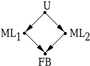
Figure 1: The causal network for ✗ ❵ and ✗ ➎ .

❍ ⑧ ✘ ➇ ML ❵ ✠ FB ➊ , so ❍ ❻ ✘ ➇ ML ➎ ➊ . It is easy to see that the contingency ML ➎ ✘ ❇ satisfies the two conditions in AC2. AC2(a) is satisfied because, in the absence of the second arsonist (ML➎ ✘ ❇ ), the first arsonist is necessary and sufficient for the fire to occur ✝ FB ✘ ❆ ✎ . AC2(b) is satisfied because, if the first match is lit (ML ❵ ✘ ❆ ) the contingencyML ➎ ✘ ❇ does not prevent the fire from burning the forest. Thus, ML ❵ ✘ ❆ is a cause of FB ✘ ❆ in ✗ ❵ . (Note that we needed to set ML➎ to 0, contrary to facts, in order to reveal the latent dependence of FB on ML ❵ . Such a setting constitutes a structural change in the original model, since it involves the removal of some structural equations.) The argument that ML ❵ ✘ ❆ is also a cause of FB ✘ ❆ in ✗ ➎ is similar. (Again, taking ❍ ⑧ ✘ ➇ ML ❵ ✠ FB ➊ and ❍ ❻ ✘ ➇ ML ➎ ➊ works.)

This example also illustrates the need for the minimality condition ❶ ➝ ➞ . For example, if lighting a match qualifies as the cause of fire then lighting a match and sneezing would also pass the tests of AC1 and AC2, and awkwardly qualify as the cause of fire. Minimality serves here to strip "sneezing" and other irrelevant, over-specific details from the cause.

It might be argued that allowing disjunctive causes would be useful in this case to distinguish ✗ ❵ from ✗ ➎ as far as causality goes. A purely counterfactual definition of causality would make ML ❵ ✘ ❆ ➠ ML ➎ ✘ ❆ a cause of FB ✘ ❆ in ✗ ❵ (since, if ML ❵ ✘ ❆ ➠ ML ➎ ✘ ❆ were not true, then FB ✘ ❆ would not be true), but would make neither ML ❵ ✘ ❆ nor ML ➎ ✘ ❆ individually a cause (for example, if ML ❵ ✘ ❆ were not true in ✗ ❵ , FB ✘ ❆ would still be true). Clearly, our definition does not enforce this intuition. Purely counterfactual definitions of causality have other well-known problems. We do not have a strong intuition as to the best way to deal with disjunction in the context of causality, and believe that disallowing it is reasonably consistent with intuitions. Interestingly, as we shall see in Section 3.2, our definition of explanation does distinguish ✗ ❵ from ✗ ➎ ; each of ML ❵ ✘ ❆ and ML ➎ ✘ ❆ is an explanation of FB ✘ ❆ in ✗ ❵ under our definition of explanation, but neither is an explanation of FB ✘ ❆ in ✗ ➎ . In ✗ ➎ , the explanation of FB ✘ ❆ is ML ❵ ✘ ❆ ❹ ML ➎ ✘ ❆ : both matches being lit are necessary to explain the forest burning down.

3.2 The Basic Definition of Explanation

All that remains to do before giving the definition of explanation is to discuss how to capture the agent's epistemic state in our framework. For ease of exposition, we first consider the case where the causal model is known and the context is uncertain. (The minor modifications required to deal with the general case are described in Section 3.4.) In that case, one way of describing an agent's epistemic state is by simply describing the set of contexts the agent considers possible. This choice is very much in the spirit of the standard "possible worlds" definitions of knowledge and belief.

Definition 3.3: (Explanation) Given a structural model ✗ , ❍ ✜ ✘ ❍ a80 is an explanation of ❧ relative to a set ➦ of contexts if the following conditions hold:

EX1. ✝ ✗ ✠ ❍ ■ ✎ ❳ ✘ ❧ for each context ❍ ■ ✒ ➦ . (That is, ❧ must hold in all contexts the agent considers possible-the agent considers what she is trying to explain as an established fact)

EX2. ❍ ✜ ✘ ❍ a80 is a weak cause of ❧ in ✝ ✗ ✠ ❍ ■ ✎ (that is, AC1 and AC2 hold, but not necessarily AC3) for each ❍ ■ ✒ ➦ such that ✝ ✗ ✠ ❍ ■ ✎ ❳ ✘ ❍ ✜ ✘ ❍ a80 .

EX3. ❍ ✜ is minimal; no subset of ❍ ✜ satisfies EX2.

EX4. ✝ ✗ ✠ ❍ ■ ✎ ❳ ✘ ➅ ✝ ❍ ✜ ✘ ❍ a80 ✎ for some ❍ ■ ✒ ➦ and ✝ ✗ ✠ ❍ ■ ❽ ✎ ❳ ✘ ❍ ✜ ✘ ❍ a80 for some ❍ ■ ❽ ✒ ➦ . (This just says that the agent considers a context possible where the explanation is false, so the explanation is not known to start with, and considers a context possible where the explanation is true, so that it is not vacuous.)

Our requirement EX4 that the explanation is not known may seem incompatible with linguistic usage. Someone discovers some fact ❶ and says "Aha! That explains why ❷ happened." Clearly, ❶ is not an explanation of why ❷ happened relative to the epistemic state after ❶ has been discovered, since at that point ❶ is known. However, ❶ can legitimately be considered an explanation of ❷ relative to the epistemic state before ❶ was discovered.

Consider the arsonists in Example 3.2. If the causal model has only arsonists as the cause of the fire, there are two possible explanations in the disjunctive scenario: arsonist 1 did it or arsonist 2 did it (assuming ➦ consists of three contexts, where either 1, 2, or both set the fire). In the conjunctive scenario, no explanation is necessary, since the agent knows that both arsonists must have lit a match if arson is the only possible cause of the fire (assuming that the agent considers these to be the only possible arsonists).

Perhaps more interesting is to consider a causal model with other possible causes, such as lightning and unattended campfires. Since the agent knows that there was a fire, in each of the contexts in ➦ , at least one of the potential causes must have actually occurred. If we assume that there is a context where only arsonist 1 lit the fire (and, say, there was lightning) and another where only arsonist 2 lit the fire then, in the conjunctive scenario, ML ❵ ✘ ❆ ❹ ML ➎ ✘ ❆ is an explanation of FB ✘ ❆ , but neither ML ❵ ✘ ❆ nor ML ➎ ✘ ❆ by itself is an explanation (since neither by itself is a cause in all contexts in ➦ that satisfy the formula). On the other hand, in the disjunctive scenario, both ML ❵ ✘ ❆ and ML ➎ ✘ ❆ are explanations.

It is worth noting here that the minimality clause EX3 applies to all contexts. This means that our rough gloss of ❍ ✜ ✘ ❍ a80 being an explanation of ❧ relative to a set ➦ of contexts if ❍ ✜ ✘ ❍ a80 is a cause of ❧ in each context in ➦ where ❍ ✜ ✘ ❍ a80 holds is not quite correct. For example, although ML ❵ ✘ ❆ ❹ ML ➎ ✘ ❆ is an explanation of fire in the conjunctive scenario (if ➦ includes contexts where there are other possible causes of fire), it is a cause of fire in none of the contexts in which it holds. The minimality condition AC3 would say that each of ML ❵ ✘ ❆ and ML ➎ ✘ ❆ is a cause, but their conjunction is not.

Note that, as for causes, we have disallowed disjunctive explanations. Here the motivation is less clear cut. It does make perfect sense to say that the reason that ❧ happened is either ❶ or ❷ (but I don't know which). There are some technical difficulties with disjunctive explanations, which suggest philosophical problems. For example, consider the conjunctive scenario of the arsonist example again. Suppose that the structural model is such that the only causes of fire are the arsonists, lightning, and unattended campfires and that ➦ consists of contexts where each of these possibilities is the actual cause of the fire. Once we allow disjunctive explanations, what is the explanation of fire? One candidate is "either there were two arsonists or there was lightning or there was an unattended campfire (which got out of hand)". But this does not satisfy EX4, since the disjunction is true in every context in ➦ . On the other hand, if we do not allow the disjunction of all possible causes, which disjunction should be allowed as an explanation? As a technical matter, how should the minimality condition EX3 be rewritten? We could not see any reasonable way to allow some disjunctions in this case without allowing the disjunction of all causes (which will not in general satisfy EX4).

We believe that, in cases where disjunctive explanations seem appropriate, it is best to capture this directly in the causal model by having a variable that represents the disjunction. (Essentially the same point is made in [Chajewska and Halpern, 1997].) For example, consider the disjunctive scenario of the arsonist example, where there are other potential causes of the fire. If we want to allow "there was an arsonist" to be an explanation without specifically mentioning who the arsonist is, then it can be easily accomplished by replacing the variables ML ❵ and ML ➎ in the model by a variable ML which is 1 iff at least one arsonist drops a match. Then ML ✘ ❆ becomes an explanation, without requiring disjunctive explanations.

Why not just add ML to the model rather than using it to replace ML ❵ and ML ➎ ? We have implicitly assumed in our framework that all possible combinations of assignments to the variables are possible (i.e., there is a structural contingency for any setting of the variables). If we add ML and view it as being logically equivalent toML ❵ ➠ ML ➎ (that is, ML ✘ ❆ by definition iff at least one of ML ❵ and ML ➎ is 1) then, for example, it is logically impossible for there to be a structural contingency where ML ❵ ✘ ❇ , ML ➎ ✘ ❇ , and ML ✘ ❆ . Thus, in the presence of logical dependences, it seems that we need to restrict the set of contingencies that can be considered to those that respect the dependencies. We have not yet considered the implications of such a change for our framework, so we do not pursue the matter here.

3.3 Partial Explanations and Explanatory Power

Not all explanations are considered equally good. Some explanations are more likely than others. An obvious way to define the "goodness" of an explanation is by bringing probability into the picture. Suppose that the agent has a probability on the set ➦ of possible contexts. In this case, we can consider the probability of the set of contexts where the explanation ❍ ✜ ✘ ❍ a80 is true. For example, if the agent has reason to believe that the first arsonist is extremely unlikely to have caused the fire (perhaps he had defective matches), then the set of contexts where ML ➎ ✘ ❆ holds would have higher probability than those where ML ❵ ✘ ❆ holds. Thus, ML ➎ ✘ ❆ would be considered a better explanation of the fire in the disjunctive model than ML ❵ ✘ ❆ .

But the probability of an explanation is only part of the story; the other part concerns the degree to which an explanation fulfills its role (relative to ❧ ) in the various contexts considered. This becomes clearer when we consider partial explanations. The following example, taken from [G¨ ardenfors, 1988], is one where partial explanations play a role.

Example 3.4: Suppose I see that Victoria is tanned and I seek an explanation. Suppose that the causal model includes variables for "Victoria took a vacation in the Canary Islands", "sunny in the Canary Islands", and "went to a tanning salon". The set ➦ includes contexts for all settings of these variables compatible with Victoria being tanned. Note that, in particular, there is a context where Victoria both went to the Canaries (and didn't get tanned there, since it wasn't sunny) and to a tanning salon. G¨ ardenfors points out that we normally accept "Victoria took a vacation in the Canary Islands" as a satisfactory explanation of Victoria being tanned and, indeed, according to his definition, it is an explanation. Victoria taking a vacation is not an explanation (relative to the context ➦ ) in our framework, since there is a context ❍ ■ ➁ ✒ ➦ where Victoria went to the Canary Islands but it was not sunny, and in ❍ ■ ➁ the actual cause of her tan is the tanning salon, not the vacation.

For us, the explanation would have to be "Victoria went to the Canary Islands and it was sunny." In this case we can view "Victoria went to the Canary Islands" as a partial explanation (in a formal sense to be defined below).

In Example 3.4 the partial explanation can be extended to a full explanation by adding a conjunct. But not every partial explanation can be extended to a full explanation. Roughly speaking, the full explanation may involve exogenous factors, which are not permitted in explanations. Assume, for example, that going to a tanning salon was not considered an endogenous variable in our model but, rather, the model simply had an exogenous variable ✱ ➫ that could make Victoria suntanned even in the absence of sun in Canary islands. Likewise, assume that the weather in Canary island was also part of the background context. In this case, we would still consider Victoria's vacation to provide a partial explanation of her sun tan, since the context where it fails to be a cause (no sun in the Canary island) is fairly unlikely, but we cannot add conjuncts to this event to totally exclude that context from the agent's realm of possibilities.

The situation actually is quite common, as the following example shows.

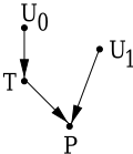
Example 3.5: Suppose that the sound on a television works but there is no picture. Furthermore, the only cause of there being no picture that the agent is aware of is the picture tube being➭ faulty. However, the agent is also aware that there are times when there is no picture even though the picture tube works perfectly well-intuitively, "for inexplicable reasons". This is captured by the causal network described in Figure 2, where ➯ describes whether or not the picture tube is working (1 if it is and 0 if it is not) and ➲ describes whether or not there is a picture (1 if there is and 0 if there is not). The ex-

1

P

Figure 2: The television with no picture.

ogenous variable ✱ ➈ determines the status of the picture tube: ➯ ✘ ✱ ➈ . The exogenous variable ✱ ❵ is meant to represent the mysterious "other possible causes". If ✱ ❵ ✘ ❇ , then whether or not there is a picture depends solely on the status of the picture tube-that is, ➲ ✘ ➯ . On the other hand, if ✱ ❵ ✘ ❆ , then there is no picture (➲ ✘ ❇ ) no matter what the status of the picture tube. Thus, in contexts where ✱ ❵ ✘ ❆ , ➯ ✘ ❇ is not a cause of ➲ ✘ ❇ . Now suppose that ➦ includes a context ❍ ■ ➈ ➈ where ✱ ➈ ✘ ✱ ❵ ✘ ❇ . Then it is easy to see that there is no explanation of ➲ ✘ ❇ . The only plausible explanation, that the picture tube is not working, is not a cause of ➲ ✘ ❇ in the context ❍ ■ ➈ ➈ . On the other hand, ➯ ✘ ❇ is a cause of ➲ ✘ ❇ in all other contexts in ➦ satisfying ➯ ✘ ❇ . If the probability of ❍ ■ ➈ ➈ is small (capturing the intuition that it is unlikely that more than one thing goes wrong with a television at once), then we are entitled to view ➯ ✘ ❇ as a quite good partial explanation of ➲ ✘ ❇ .

These examples motivate the following definition.

Definition 3.6: Let ➦ ◗ ✣ ➵ ◗ ❚ ➸ ➺ be the largest subset ➦ ❽ of ➦ such that ❍ ✜ ✘ ❍ a80 is an explanation of ❧ relative to ➦ ◗ ✣ ➵ ◗ ❚ ➸ ➺ . (It is easy to see that there is a largest such set.) Then ❍ ✜ ✘ ❍ a80 is a partial explanation of ❧ with goodness ➻ ➼ ✝ ➦ ◗ ✣ ➵ ◗ ❚ ➸ ➺ ❳ ❍ ✜ ✘ ❍ a80 ✎ . Thus, the goodness of a partial explanation measures the extent to which it provides an explanation of ❧ . 1

In Example 3.4, if the agent believes that it is sunny in the Canary Islands with probability .9 (that is, the probability that it was sunny given that Victoria is suntanned and that she went to the Canaries is .9), then Victoria going to the Canaries is a partial explanation of her being tanned with goodness .9. The relevant set ➦ ❽ consists of those contexts where it is sunny in the Canaries. Similarly, in Example 3.5, if the agent believes that the probability of both the picture tube being faulty and the other mysterious causes being operative is .1, then ➯ ✘ ❇ is a partial explanation of ➲ ✘ ❇ with goodness .9 (with ➦ ❽ consisting of all the contexts where ✱ ❵ ✘ ❆ ).

1 Here and elsewhere, a formula such as ➽ ➾ ➚ ➽ ➶ is being identified with the set of contexts where the formula is true. Recall that, since all contexts in ➹ are presumed to satisfy ➘ , there is no need to condition on ➘ ; this probability is already updated with the truth of the explanandum ➘ . Finally, note that our usage of partial explanation is related to, but different from, that in [Chajewska and Halpern, 1997].

A full explanation is clearly a partial explanation with goodness 1, but we are often satisfied with partial explanations ❍ ✜ ✘ ❍ a80 that are not as good, especially if they have high probability (i.e., if ➻ ➼ ✝ ❍ ✜ ✘ ❍ a80 ✎ is high). In general, there is a tension between the goodness of an explanation and its probability.

These ideas also lead to a definition of explanatory power. Consider Example 3.2 yet again, and suppose that there is an endogenous random variable ➴ corresponding to the presence of oxygen. Now if ➴ ✘ ❆ holds in all the contexts that the agent considers possible, then ➴ ✘ ❆ is excluded as an explanation by EX4. But suppose that ➴ ✘ ❇ holds in one context that the agent considers possible (for example, there may be another combustible gas), albeit a very unlikely one. In that case, ➴ ✘ ❆ becomes a very good partial explanation of the fire. Nevertheless, it is an explanation with, intuitively, very little explanatory power. How can we make this precise?

Suppose that there is a probability distribution ➻ ➼ ✷ on a set ➦ ✷ of contexts larger than ➦ that intuitively represents the agent's prior probability before the explanandum ❧ is discovered. That is, ➻ ➼ is the result of conditioning ➻ ➼ ✷ on ❧ and ➦ consists of the subset of ➦ ✷ that satisfies ❧ . G¨ ardenfors identifies the explanatory power of the (partial) explanation ❍ ✜ ✘ ❍ a80 of ❧ with ➻ ➼ ✷ ✝ ❧ ❳ ❍ ✜ ✘ ❍ a80 ✎ (see [Chajewska and Halpern, 1997; G¨ ardenfors, 1988]). If this probability is higher than ➻ ➼ ✷ ✝ ❧ ✎ , then the explanation makes ❧ more likely. While this explanatory power, we would argue that a better measure of the explanatory power of ❍ ✜ ✘ ❍ a80 is ➻ ➼ ✷ ✝ ➦ ◗ ✣ ➵ ◗ ❚ ➸ ➺ ❳ ❍ ✜ ✘ ❍ a80 ✎ . According to either definition, under reasonable assumptions about ➻ ➼ ✷ , ➴ ✘ ❆ has much lower explanatory power than, say ML ✘ ❆ . Moreover, the two definitions agree in the case that ❍ ✜ ✘ ❍ a80 is a full explanation (since then ➦ ◗ ✣ ➵ ◗ ❚ ➸ ➺ is just ➦ , the set of contexts in ➦ ✷ where ❧ is true). The difference between the two definitions arises if there are contexts where ❧ and ❍ ✜ ✘ ❍ a80 both happen to be true, but ❍ ✜ ✘ ❍ a80 is not a cause of ❧ . Such spurious correlations are exculded by our suggested definition. (See [Pearl, 2000] for some examples showing that considering spurious correlations leads to bad outcomes.)

Again, (partial) explanations with higher explanatory power typically are more refined and, hence, less likely. than explanations with less explanatory power. There is no obvious way to resolve this tension. (See [Chajewska and Halpern, 1997] for more discussion of this issue.)

As this discussion suggests, our definition shares some features with that of G¨ ardenfors' 1988. Like him, we consider explanation relative to an agent's epistemic state. G¨ ardenfors also considers a "contracted" epistemic state characterized by the distribution ➻ ➼ ✷ . Intuitively, ➻ ➼ ✷ describes the agent's beliefs before discovering ❧ . (More accurately, it describes an epistemic state as close as possible to ➻ ➼ where the agent does not ascribe probability 1 to ❧ .) If the agent's current belief in ❧ came about as the result of an observation ⑩ , then we can take ➻ ➼ to be the result of conditioning ➻ ➼ ✷ on ⑩ , as we ➬ have done above. However, G¨ ardenfors does necessarily assume such a connection between ➻ ➼ and ➻ ➼ ✷ . In any case, for G¨ ardenfors, ❍ ✜ ✘ ❍ a80 is an explanation of ❧ relative to ➻ ➼ if (1) ➻ ➼ ✝ ❧ ✎ ✘ ❆ , (2) ❇ ➮ ➻ ➼ ✝ ❍ ✜ ✘ ❍ a80 ✎ ➮ ❆ , and (3) ➻ ➼ ✷ ✝ ❧ ❳ ❍ ✜ ✘ ❍ a80 ✎ ➱ ➻ ➼ ✷ ✝ ❧ ✎ . (1) is the probabilistic analogue of EX1. Clearly, (2) is the probabilistic analogue of EX4. Finally, (3) says that learning the explanation increases the likelihood of ❧ . G¨ ardenfors focuses on the explanatory power of an explanation, but does not take into account its prior probability. As pointed out in [Chajewska and Halpern, 1997], G¨ ardenfors' definition suffers from another defect: Since there is no minimality requirement like EX3, if ❍ ✜ ✘ ❍ a80 is an explanation of ❧ , so too is ❍ ✜ ✘ ❍ a80 ❹ ❍ ✑ ✘ ❍ ❜ .

In contrast to G¨ ardenfors' definition, the dominant approach to explanation in the AI literature, the maximum a posteriori (MAP) approach (see, for example, [Henrion and Druzdzel, 1990; Pearl, 1988; Shimony, 1991]), focuses on the probabability of the explanation, given the explanandum (i.e, ➻ ➼ ✷ ✝ ❍ ✜ ✘ ❍ a80 ❳ ❧ ✎ ✘ ➻ ➼ ✝ ❍ ✜ ✘ ❍ a80 ✎ ), but does not take explanatory power into account. The MAP approach is based on the intuition that the best explanation for an observation is the state of the world (in our setting, the context) that is most probable given the evidence. The most probable explanation for ❧ is then the context ❍ ■ ➁ such that ➻ ➼ ✝ ❍ ■ ➁ ✎ ✘ ✃ ❐ ❒ ◗ ❰ ➻ ➼ ✝ ❍ ■ ✎ . Thus, an explanation is a (complete) context. This means that part of the explanation will include totally irrelevant facts (the agent sneezed). Moreover, it is quite sensitive to the description of the context (see [Chajewska and Halpern, 1997] for details) and does not directly take causality into account.

To some extent, these problems can be dealt with by limiting the set of candidate explanations to ancestors (of the explanandum) in the causal network; this also avoids many of the problems associated with non-causal approaches (although it requires there to be a causal network in the background). However, the MAP approach does not go far enough. One problem is that propositions with extremely high prior probabilities (e.g., that oxygen is present in the room) will also receive high posterior probabilities, regardless of how relevant they are to the events explained. To remedy this problem, more intricate combinations of the quantities ➻ ➼ ✝ ❍ ✜ ✘ ❍ a80 ✎ , ➻ ➼ ✷ ✝ ❧ ❳ ❍ ✜ ✘ ❍ a80 ✎ , and ➻ ➼ ✷ ✝ ❧ ✎ have been suggested to quantify the causal relevance of ❍ ✜ ✘ ❍ a80 on ❧ but, as argued in [Pearl, 2000, p. 221], without taking causality into account, no such combination of parameters can work.

3.4 The General Definition

In general, an agent may be uncertain about the causal model, so an explanation will have to include information about it. (G¨ ardenfors 1988 and Hempel 1965 make similar observations). It is relatively straightforward to extend our definition of explanation to accommodate this. Now an epistemic state ➦ consists not only of contexts, but of pairs ✝ ✗ ✠ ❍ ■ ✎ consisting of a causal model ✗ and a context ❍ ■ . Call such a pair a situation. Intuitively, now an explanation should consist of some causal information (such as "prayers do not cause fires") and the facts that are true. Thus, a (general) explanation has the form ✝ ⑩ ✠ ❍ ✜ ✘ ❍ a80 ✎ , where ⑩ is an arbitrary formula in our causal language and, as before, ❍ ✜ ✘ ❍ a80 is a conjunction of primitive events. We think of the ⑩ component as consisting of some causal information (such as "prayers do not cause fires", which corresponds to a conjunction of statements of the form ✢ ✘ ✇ a207 ❴ ➲ ❛ a80 ❥ ✝ ✢ ✘ ✇ ✎ , where ➲ is a random variable describing whether or not prayer takes place). The first component in a general explanation is viewed as restricting the set of causal models. To make this precise, given a causal model ✗ , we say ⑩ is valid in ✗ , and write ✗ ❳ ✘ ⑩ , if ✝ ✗ ✠ ❍ ■ ✎ ❳ ✘ ⑩ for all contexts ❍ ■ consistent with ✗ . With this background, it is easy to state the general definition.

Definition 3.7: ✝ ⑩ ✠ ❍ ✜ ✘ ❍ a80 ✎ is an explanation of ❧ relative to a set ➦ of situations if the following conditions hold:

EX3. ✝ ⑩ ✠ ❍ ✜ ✘ ❍ a80 ✎ is minimal; there is no pair ✝ ⑩ ❽ ✠ ❍ ✜ ❽ ✘ ❍ a80 ❽ ✎ a209 ✘ ✝ ⑩ ✠ ❍ ✜ ✘ ❍ a80 ✎ satisfying EX2 such that ➇ ✗ ❽ ❽ ✒ ✗ ✝ ➦ ✎ ✦ ✗ ❽ ❽ ❳ ✘ ⑩ ❽ ➊ a210 ➇ ✗ ❽ ❽ ✒ ✗ ✝ ➦ ✎ ✦ ✗ ❽ ❽ ❳ ✘ ⑩ ➊ , where a212 ✝ ➦ ✎ ✘ ➇ ✗ ✦ ✝ ✗ ✠ ❍ ■ ✎ ✒ ➦ for some ❍ ■ ➊ , ❍ ✜ ❽ ❼ ❍ ✜ , and ❍ a80 ❽ is the restriction of ❍ a80 to the variables in ❍ ✜ ❽ . Roughly speaking, this says that no subset of ✜ provides a weak cause of ❧ in more contexts than those where ⑩ is valid.

Note that, in EX2, we now restrict to situations ✝ ✗ ✠ ❍ ■ ✎ ✒ ➦ that satisfy both parts of the explanation ✝ ⑩ ✠ ❍ ✜ ✘ ❍ a80 ✎ , in that ✗ ❳ ✘ ⑩ and ✝ ✗ ✠ ❍ ■ ✎ ❳ ✘ ❍ ✜ ✘ ❍ a80 . Furthermore, although both components of an explanation are formulas in our causal language, they play very different roles. The first component serves to restrict the set of causal models considered (to those with the appropriate structure); the second describes a cause of ❧ in the resulting set of situations.

Clearly Definition 3.3 is the special case of Definition 3.7 where there is no uncertainty about the causal structure (i.e., there is some ✗ such that if ✝ ✗ ❽ ✠ ❍ ■ ✎ ✒ ➦ , then ✗ ✘ ✗ ❽ ). In this case, it is clear that we can take ⑩ in the explanation to be true.

Definition 3.7 can also be extended to deal naturally with statistical information of the kind considered by G¨ ardenfors and Hempel. Let a probabilistic causal model be a tuple ✗ a214 a215 ✘ ✝ ✆ ✠ ✚ ✠ ➻ ➼ ✎ , where ✗ ✘ ✝ ✆ ✠ ✚ ✎ is a causal model and ➻ ➼ is a probability measure on the contexts defined by signature ✆ of ✗ . Information like "with probability .9, ✜ ✘ ➞ " is a restriction on probabilistic models, and thus can be captured using a formula in an appropriate extension of our language that allows such probabilistic reasoning. With this extended language, the definition of explanation using probabilistic causal models remains unchanged.

As an orthogonal issue, there is also no difficulty considering a probability on the set ➦ of situations and defining partial explanation just as before.

Example 3.8: Using this general definition of explanation, consider Scriven's 1959 famous paresis example. Paresis develops only in patients who have been syphilitic for a long time, but only a small number of patients who are syphilitic in fact develop paresis. Furthermore, according to Scriven, no other factor is known to be relevant in the development of paresis. 2 This description is captured by a simple causal model ✗ a214 . There are two endogenous variables, a217 (for syphilis) and ➲ (for paresis), and two exogenous variables, ✱ ❵ , the background factors that determine a217 , and ✱ ➎ , which intuitively represents "disposition to paresis", i.e., the factors that determine, in conjunction with syphilis, whether or not paresis actually develops. An agent who knows this causal model and that a patient has paresis does not need an explanation of why: the agent knows without being told that the patient must have syphilis and that ✱ ➎ ✘ ❆ . On the other hand, for an agent who does not know the causal model (i.e., considers a number of causal models of paresis possible), ✝ ➇ ✗ a214 ➊ ✠ a217 ✘ ❆ ✎ is an explanation of paresis.

4 Discussion

We have given a formal definition of explanation in terms of causality. As we mentioned earlier, there are not too many formal definitions of explanation in terms of causality in the literature. One of the few exceptions is Lewis 1986a, who defends the thesis that "to explain an event is to provide some information about its causal history". While this view is compatible with our definition, there is no formal definition given to allow for a careful comparison between the approaches. In any case, if were to define causal history in terms of Lewis's 1986b definition of causality, we would inherit all the problems of that definition. As we said earlier, our definition avoids these problems.

So what are the problems with our definition? For one thing, it inherits whatever problems our definition of causality has. As observed in [Halpern and Pearl, 2001], our definition at times declares certain events to be causes (and hence candidate explanations) that, intuitively, should not be causes because they should fail AC2(a). The only reason that they do not fail AC2(a) is because of extremely unlikely structural contingencies. To some extent, we can avoid this problem by simply ignoring structural contingencies that are extremely unlikely (this is essentially the solution suggested in [Halpern and Pearl, 2001] in the context of causality). Of course, we can do this in the context of explanation too. Another possibility is to take the probability of the structural contingency into account more directly when computing the probability of the explanation. We are currently exploring this option.

We have mentioned the other significant problem of the definition already: dealing with disjunctive explanations. Disjunctions cause problems in the definition of causality, which is why we do not deal with them in the context of explanation. As we pointed out earlier, it may be possible to modify the definition of causality so as to be able to deal with conjunctions without changing the structure of our definition of explanation. We are currently exploring this.

2 Apparently there are now other known factors, but this does not change the import of the example.

Finally, our definition gives no tools for dealing with the inherent tension between explanatory power, goodness of partial beliefs, and the probability of the explanation. Clearly this is an area that requires further work.

Acknowledgments:

Thanks to Riccardo Pucella and Vicky Weissman for useful comments.