Ambiguity-Directed Sampling for Qualitative Analysis of Sparse Data from Spatially-Distributed Physical Systems

1 Introduction

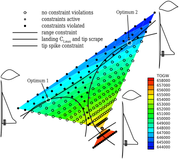
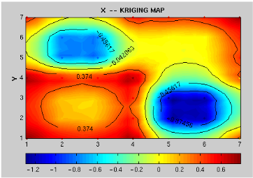
A number of important scientific and engineering applications, such as fluid dynamics simulation and aircraft design, require qualitative analysis of spatially-distributed data from expensive experiments and/or complex simulations demanding days, weeks, or even years on petaflops-class computing systems. For example, Fig. 1 shows a cross-section of the design space for a multidisciplinary aircraft design problem involving 29 design variables with 68 constraints in a highly non-convex design space [Knill et al., 1999]. Frequently, the designer will change some aspect of a nominal design point, and run a simulation to see how the change affects the objective function and various constraints dealing with aircraft geometry and performance/aerodynamics. This approach is inadequate for exploring such large high-dimensional design spaces, even at low fidelity. Ideally, the design engineer would like a high-level mining system to identify the pockets that contain good designs and which merit further consideration; traditional tools from optimization and approximation theory can then be applied to fine-tune such preliminary analyses.

Two important characteristics distinguish these applications. First, they must deal not with an abundance of data, but rather with a scarcity of data, owing to the cost and time

Naren Ramakrishnan

Virginia Tech Dept. of Computer Science 629 McBryde Hall Virginia Tech, VA 24061 naren@cs.vt.edu

involved in conducting simulations. Second, and more importantly, the computational scientist has complete control over the data acquisition process (e.g. regions of the design space where data can be collected), especially via computer simulations. It is natural therefore to focus data collection so as to maximize information content, minimize the number and expense of samples, and so forth.

This paper presents a principled mechanism for applying domain-specific knowledge to focus sampling strategies for data-scarce applications. In particular, ambiguities identified by a multi-level qualitative analysis of data collected in one iteration guide succeeding iterations of data collection so as to improve the qualitative analysis. This approach leads to highly effective sampling decisions that are explainable in terms of problem structures and domain knowledge. We demonstrate the effectiveness of our approach by two case studies: (1) identification of pockets in n-dimensional space, and (2) decomposition of a field based on control influences.

2 Qualitative Analysis of Spatially-Distributed Physical Systems

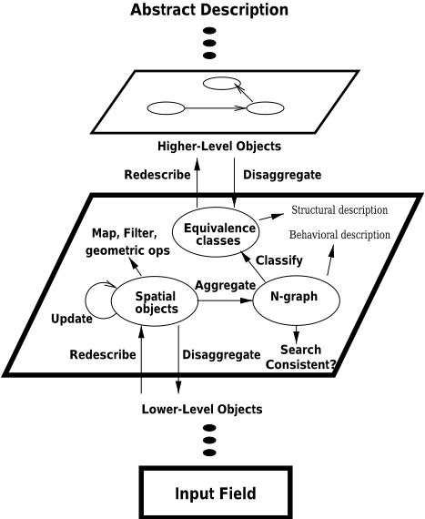
The mechanism we develop for ambiguity-directed sampling is based on the Spatial Aggregation Language (SAL) [Bailey- Kellogg et al., 1996; Yip and Zhao, 1996], which supports construction of data interpretation and control design applications for spatially-distributed physical systems. SAL programs uncover and manipulate multi-layer geometric and topological structures in spatially distributed data by using a small number of uniform operators and data types, parameterized by domain-specific knowledge. These operators and data types mediate increasingly abstract descriptions of the input data, as shown in Fig. 2. They utilize knowledge of physical properties such as continuity and locality, based on specified metrics, adjacency relations, and equivalence predicates, to uncover regions of uniformity in spatially distributed data.

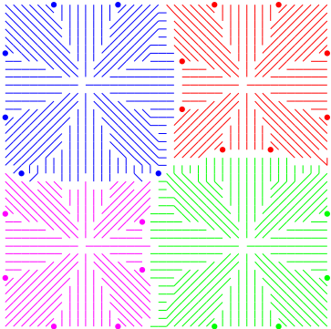
As an example (see Fig. 3), consider a SAL program for bundling the vectors in a given vector field (e.g. wind velocity or temperature gradient) into a set of streamlines (paths through the field following the vector directions):

1. Aggregate vectors into a neighborhood graph (say 8adjacency), localizing computation.
2. Filter edges in the graph, ensuring edge direction is similar enough to vector direction.
3. Cluster into equivalence classes neighboring vectors whose directions match best.
4. Redescribe equivalence classes of vectors into more abstract streamline curves.

In a second level of abstraction, streamlines are aggregated and classified into groups with similar flow behavior

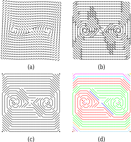
(Fig. 3(d)), using the exact same operators but with different metrics. As this example illustrates, SAL provides a vocabulary for expressing the knowledge required - distance metrics, similarity metrics, etc. - for uncovering multi-level structures in spatial data sets. It has been applied to applications ranging from decentralized control design [BaileyKellogg and Zhao, 1999; 2001] to analysis of diffusionreaction morphogenesis [Ord´o˜nez and Zhao, 2000].

3 Ambiguity-Directed Sampling

We extend SAL for data-scarce, rather than data-rich, applications, by focusing data collection in areas that will yield information most useful in discriminating among possible models. Given a set of possible SAL models M = {m1, m2, . . . , mn} for the data, we want to choose a new sample s to help discriminate among posterior probabilities P(mi | s). For instance, in the vector-bundling example (Fig. 3), models would represent different choices of how to group vectors into streamlines. By Bayes rule, we need to evaluate P(s |mi) and P(mi). The domain knowledge used to enumerate the possible SAL structures also places priors P (mi) on the identified models. In the vector-bundling example, a possible streamline can be scored based on how well its curvature matches the directions of the vectors it aggregates. Additional domain knowledge then characterizes the dependence of potential sample values on different models, thus helping to optimize the next sample location. As we will show later in this section, one useful form of such dependence relates to addressing ambiguity. For example, the best aggregation for ambiguous streamlines can be determined by sampling the interpolate : field × new objects × surrogate→new values Determine values for new objects based on values for nearby objects in field, according to surrogate function.

classify : objects × equiv predicate→classes × ambiguities

Apply predicate to neighboring objects, partitioning them into equivalence classes and left-over ambiguous objects. Predicate is a function taking a pair of neighbors and returning one of {true, false, ambiguous}.

sample : objects × ambiguities × objective fn→new objects Determine new objects to be sampled based on optimization of an objective function indicating information gain with respect to the ambiguities.

Table 1: Ambiguity-directed sampling operators.

flow near streamline "branch points."

Tab. 1 summarizes the incorporation of domain knowledge in new SAL operators by our ambiguity-directed sampling framework. The data interpretation and sampling process proceeds as follows, starting from some initial sparse data. (1) Derive qualitative SAL structures from either the sparse data, or a dense dataset interpolated with a surrogate function. (2) Identify ambiguities arising in the structure formation process. (3) Target a sample point that will optimize the information gain with respect to these ambiguities. (4) Update the data set and repeat, as long as information gain is substantial enough. The following subsections describe the key parts of this approach in more detail.

3.1 Interpolation with a Surrogate Function

In some cases it is advantageous to generate a dense dataset and find structures in it, rather than to work directly from sparse data. For example, when possible models have a known, common structure (e.g. they can be treated as locally smooth quadratic functions), then interpolating dense data can simplify structure and ambiguity identification. The interpolate operator in Tab. 1 generates such dense data, according to a given surrogate representation.

The choice of surrogate representation is constrained by the local nature of SAL computations. For example, global, least-squares type approximations are inappropriate since measurements at all locations are equally considered to uncover trends and patterns in a particular region. We advocate the use of kriging-type interpolators [Sacks et al., 1989], which are local modeling methods with roots in Bayesian statistics. Kriging can handle situations with multiple local extrema (for example, in weather data, remote sensing data, etc.) and can easily exploit anisotropies and trends. Given k observations, the interpolated model gives exact responses at these k sites and estimates values at other sites by minimizing the mean squared error (MSE), assuming a random data process of known functional form.

Formally (for two dimensions), the true function p is assumed to be the realization of a random process such as:

where β is typically a uniform random variate, estimated based on the known k values of p, and Z is a correlation function with zero mean and known variance. Kriging then estimates a model p′ of the same form, based on the k observations:

and minimizing mean squared error between p′ and p:

A typical choice for Z in p′ is σ2R, where scalar σ2 is the estimated variance, and the symmetric correlation matrix R can encode domain-specific constraints and factors reflecting the current fidelity of data. We use an exponential function for entries in R, with two parameters C1 and C2:

Intuitively, function estimation at a given point is influenced more by observations nearby than by those farther away.

The estimator minimizing mean squared error is then obtained by multi-dimensional optimization:

This expression can be derived from the conditions that there is no error between the model and the true values at the chosen k sites, and that all variability in the model arises from the design of Z (the derivation is beyond the scope of this paper). The multi-dimensional optimization is often performed by gradient descent or pattern search methods. More details are available in [Sacks et al., 1989], which demonstrates this methodology in the context of the design and analysis of computer experiments.

3.2 Bottom-Up Detection of Ambiguity

The SAL equivalence class clustering mechanism (operating on the sparse input data or the dense surrogate model) exploits continuity, grouping neighboring objects that satisfy a domain-specific equivalence predicate (e.g. similar vector direction). At discontinuities, dissimilar neighboring objects are placed in separate classes. However, within a weakly-similar class or across a weakly-different discontinuity, neighboring objects might almost satisfy the predicate. For example, some vectors in Fig. 3(b) have two possible forward neighbors; in some cases, a vector might equally well belong to either of two flows. We call such unclear classification choice points ambiguous.

The bottom-up SAL operators introduced in Sec. 2 can be used to detect ambiguities if the equivalence class clustering operator classify is extended as in Tab. 1. In particular, a domain-specific equivalence predicate indicates when neighbors are equivalent, not equivalent, or ambiguous, allowing classify to delay ambiguous classification decisions.

3.3 Top-Down Utilization of Ambiguity

Ambiguity can reflect the desirability of acquiring data at or near a specified point, to clarify the correct classification and to serve as a mathematical criterion of information content. The sample operator specified in Tab. 1 addresses this opportunity by generating samples to optimize a given domain-specific objective function, given a set of ambiguous objects. For example, in response to a vector with an ambiguous neighbor, it might suggest nearby locations to sample. In other applications, it might pick the midpoint between a pair of ambiguous points, or even (see the influence-based model decomposition application below) apply SAL recursively to qualitatively analyze a set of ambiguous points. In conjunction with a surrogate function, some functional of the MSE (Eq. 3) can be used to focus sampling, by a suitable statistical design. 1 Section 4.2 describes the use of such an objective function.

When using a surrogate function, the correlation matrix R (Eq. 4) can be modified to emphasize the desirability of focusing the fitting effort on ambiguous regions. In particular, indicator covariance terms modulate R when the standard uniformly parameterized model (C1 and C2 in our case) does not adequately capture the observed variability. Our approach is reminiscent of incorporating "Type C soft data" into variogram estimation [Journel, 1986]: "soft" data have nonnegligible uncertainty and "Type C" data are obtained without additional experimentation (in our case, via SAL analysis). By using the pcdf of ambiguous objects as an indicator covariance term, we can improve covariance estimates, and also help suggest data locations that will clarify the correct classification. The exact equations are beyond the scope of this article, but we refer the reader to [Journel, 1986] for an account of this "soft kriging" approach.

3.4 Iteration

Data are collected for the indicated sample points, by experiment or simulation. When a surrogate function is used, the fitted model is refined with real data at the indicated points, via interpolate. We note that efficient implementations of some data structures (e.g. Delaunay triangulation neighborhood graphs) can be incrementally updated with the additional samples [Ord´o˜nez and Zhao, 2000]. The aggregation process can then be repeated with the extended data set, terminating when the information-theoretic metric used by sample drops below some specified level.

4 Applications

This section discusses how the computational framework of two existing applications can be redescribed in terms of ambiguity-directed sampling, and then illustrates the effectiveness of our approach with two new case studies.

4.1 Existing Applications

KAM [Yip, 1991] interprets the behaviors of Hamiltonian dynamical systems by phase-space analysis. Geometric points represent states of the system for a given set of parameters. KAM works directly with these samples - it does not interpolate a dense representation. KAM groups points into orbits describing the system's temporal evolution; it groups orbits into phase portraits describing evolution of all states for a given set of parameters; and it groups phase portraits into bifurcation maps describing variations in portraits due to variations in parameters. At each stage, KAM adds samples when it detects an inadequate description. In our vocabulary, the classify predicate clustering orbits into a phase portrait notices when two neighboring orbits cannot physically be adjacent; sample then starts orbit integration from the mid-point of an ambiguous pair of neighboring points. Similarly, in a bifurcation map additional phase portraits are generated for parameter values between those of ambiguous neighboring phase portraits.

1 Sample selection optimization is different from kriging interpolation optimization (Eq. 5), used to generate a dense data field.

STA [Ord´o˜nez and Zhao, 2000] has been applied to build high-level descriptions of morphogenesis in diffusionreaction systems by tracking aggregates of sample "floaters" that react to changes in the underlying field. In particular, floaters attempt to ensure an adequate sampling of the field (no interpolation is required), especially in high-gradient areas. They do this in a manner similar to the particle system of Witkin and Heckbert [1994], by repelling each other, splitting, and merging. In our vocabulary, the classify predicate bundling floaters in a region tests whether or not neighboring floaters are near enough relative to an energy metric measuring adequate representation of the region; sample simply splits one ambiguous floater into two adjacent floaters.

4.2 Pocket Identification

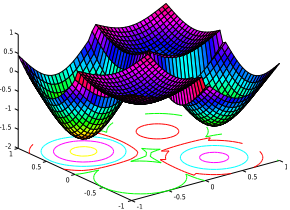
Our first application domain is motivated by research in spatial statistics [Journel, 1986; Sacks et al., 1989] and multidisciplinary system design [Knill et al., 1999]. Visualize the ndimensional hypercube defined by xi ∈ [-1, 1], i = 1 · · · n, with the n-sphere of radius 1 centered at the origin (Σxi 2 ≤ 1) embedded inside it. Notice that the ratio of the volume of the cube (2n ) to that of the sphere (πn/2 /(n/2)!) grows unboundedly with n. In other words, the volume of a highdimensional cube is concentrated in its corners (a counterintuitive notion at first). Carl de Boor exploited this property to design a difficult-to-optimize function which assumes a pocket in each corner of the cube (Fig. 4), that is just outside the sphere [Rice, 1992]. Formally, it can be defined as:

where X is the n-dimensional point (x1, x2, · · · , xn) at which the pocket function p is evaluated, I is the identity n-vector, and ‖ · ‖ is the L2 norm.

It is easily seen that p has 2n local minima; if n is large (say, 30, which means it will take more than half a million points to just represent the corners of the n-cube!), naive global optimization algorithms will require an unreasonable number of function evaluations. However, in real-world domains, significant structure exists and can often be exploited. A good example is the STAGE algorithm [Boyan and Moore, 2000], which intelligently selects starting points for local search algorithms. Our goals here are very different from global optimization: we wish to obtain a qualitative indication of the existence, number, and locations of pockets, using low-fidelity models and/or as few data points as possible. The results can then be used to seed higher-fidelity calculations. This is also fundamentally different from DACE [Sacks et al., 1989], polynomial response surface approximations [Knill et al., 1999], and other approaches in geo-statistics where the goal is accuracy of functional prediction at untested data points. Here, accuracy of estimation is traded for the ability to mine pockets.

In a dense field of data, it is straightforward to identify pockets by applying the vector field bundling implementation discussed in the introduction (see Fig. 3) to the gradient field. In the data-scarce setting, we follow the ambiguity-directed sampling framework, incorporating the domain-specific knowledge summarized in Tab. 2. Given a surrogate model, vector bundling identifies vectors which can participate in multiple good streamlines. The surrogate model incorporates these ambiguities with an indicator covariance term counting the number of possible good neighbors. This "ambiguity distribution" provides a novel mechanism to include qualitative information - streamlines that agree will generally contribute less to data mining, just as samples that are far apart are weighted less in the original R matrix. Thus, this framework can be viewed as a natural generalization of the assumptions of sample clustering that underlie kriging.

The sample objective function described in Tab. 2 minimizes the expected posterior entropy on the unsampled design space, which by a reduction argument, can be shown to be maximizing the prior entropy over the entire design space [Sacks et al., 1989]. In turn, this means that the amount of information obtained from an experiment is maximized. For our purposes, the objective function thus provides a basis to choose sample points that will improve our modeling of p.

We applied the ambiguity-driven mechanism to determining pockets in both 2D and 3D. We used a variation of the pocket function with a pseudorandom perturbation that shifts the pockets away from the corners in a somewhat unpredictable way. This twist precludes many forms of analyses, such as symbolic parsing, by imposing a highly nonlinear global map of pocket locations. In the traditional pocket function, the dips can be viewed as being influenced by little spheres at the corners, with known radii and centers. The new pocket design uses an additional parameter to impose non-symmetric perturbations which randomize both the radii and centers. As a result, local modeling must be carried out at each corner to determine the exact location of the pocket. More detail about this function can be found in [Rice, 1992,

Surrogate model

Use kriging interpolator with indicator covariance term (modeling number of similar-enough neighbors from predicate below) to estimate p at unknown points.

Vector equivalence predicate

Return true if vector directions are similar enough, false if they aren't, and ambiguous if a vector has multiple neighbors with similar-enough directions.

Sample objective function

Minimize the entropy E(-log d), where d is the conditional density of p over the design space not covered by the current data values.

Table 2: Domain knowledge for ambiguity-directed sampling in pocket identification.

pp. 113-114].

The initial experimental configuration used a face-centered design (4 points in the 2D case). The surrogate model then generated a 41n -point grid. The ambiguity-directed mechanism selected new design points, using the vector field bundling approach discussed above. Standard parameter settings were applied: required similarity of 0.8 for dot product of adjacency direction and vector field direction, and factor of 0.01∗distance penalizing the grouping of far-apart vectors.

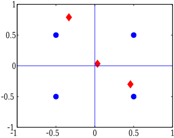
Fig. 5 shows a design involving only 7 total data points that is able to mine the four pockets. As previously discussed, our sampling decisions result in highly sub-optimal designs according to traditional metrics of variance in predicted values and D-optimality, but are sufficient to determine pockets. In particular, the ambiguity-driven framework completely skips one of the quadrants in selecting new points. This indicates that neighborhood calculations involving the other three quadrants are enough to uncover the pocket in the fourth quadrant. Since the kriging interpolator uses local modeling and since pockets in 2D effectively occupy the quadrants, obtaining measurements at ambiguous locations serves to capture the relatively narrow regime of each dip, which in turn helps to distinguish the pocket in the neighboring quadrant. This effect is hard to achieve without qualitative feedback. For higher dimensions (including 3D), the pockets move further away from the center of the design space, necessitating the sampling of points in all corners.

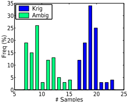
Fig. 6 shows the distributions of number of design points required for ambiguity-directed and kriging-based pocket identification over 100 perturbed variations of the 2D pocket function. Ambiguity-directed sampling required 3 to 11 additional samples, with the latter figure in the pathological case where the random perturbations cause a nearly quintic dip, rendering the initial adjacency calculations misleading. In comparison, conventional incremental kriging techniques (of the form described in Section 3.1 without qualitative analysis) required 13 to 19 additional data points. While pockets in the bigger dips are discovered quickly, the quintic and shallow dips require more function evaluations. Tests with pockets in 3D yielded even more significant results: up to 151 additional points for regular kriging, but at most 42 for ambiguitydirected sampling. With the use of block kriging, reductions in both values could be enjoyed, but these figures illustrate the effectiveness of our technique.

The extension to more than 3 dimensions is straightforward and is not detailed here for ease of presentation. It essentially entails using the appropriate covariance matrix and SAL data structures (e.g. 8-adjacency in 2D, 26-adjacency in 3D, . . . ). While we believe our ambiguity-directed framework will fare well compared to traditional kriging, a more careful study will be needed to characterize the scalability of our approach.

4.3 Influence-BasedModel Decomposition

Influence-based model decomposition [Bailey-Kellogg and Zhao, 1999; 2001] is an approach to designing spatiallydistributed data interpretation and decentralized control applications, such as thermal regulation for semiconductor wafer processing and noise control in photocopy machines. A decentralized influence graph, built by sampling the effects of controls on a field (either physically or by solving a partial differential equation), represents influences of controls on distributed physical fields. Given the expense of obtaining influence graph values, it is desirable to minimize the number of samples required. This section demonstrates that ambiguity-directed sampling can greatly reduce the number of samples required. Note that we do not interpolate a dense representation, following the explicit kriging methodology, since it sometimes does not result in explainable designs, by overlooking "nice" properties such as balance, symmetry, collapsibility, and comparability [Easterling, 1989].

Influence-based model decomposition uses influence graphs for control placement and parameter design algorithms that exploit physical knowledge of locality, linear superposability, and continuity for distributed systems with large numbers of coupled variables (often modeled by partial differential equations). By leveraging the physical knowledge encapsulated in influence graphs, these control design algorithms are more efficient than standard techniques, and produce designs explainable in terms of problem structures. Influence-based model decomposition decomposes a problem domain so as to allow relatively independent design of controls for the resulting regions. Fig. 7 overviews the approach:

1. Represent in an influence graph the effects of a few sample probe controls on the field - in this example, the heat flows induced in a piece of material by point heat sources.

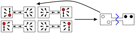
1. Cluster the probes based on similarities in their effects, as represented in the influence graph. For example, the geometric constraint imposed by the narrow channel in the dumbbell-shaped piece of material results in similar field responses to the two probes in the left half of the dumbbell and similar responses to the two probes in the right half of the dumbbell. Note that influence graphs encapsulate not only geometry but also material properties, which can greatly impact heat flows and thus the proper decomposition.
2. Cluster the field nodes based on the probe clustering, applying a predicate testing if neighboring field nodes are well-represented by the same probe nodes. In the example, the field nodes in the left half of the dumbbell are best represented by the probe nodes also in the left half (which belong to the same probe equivalence class), and are thus decomposed from the nodes in the right half. Controls are placed in the regions and optimized by a separate process not discussed here.

The quality of decompositions from a small number of randomly-placed probes is competitive with that of a spectral partition of the complete influence graph (computed following an approach developed for image segmentation [Shi and Malik, 1997]), but with orders of magnitude less computation and in a decentralized model [Bailey-Kellogg and Zhao, 2001]. We now extend this approach to show that replacing random sampling with ambiguity-directed sampling achieves even better results. Ambiguity-directed sampling effectively closes the loop between the field decomposition and influence graph sampling (dashed arrow in Fig. 7). Tab. 3 describes the the domain-specific knowledge used in ambiguitydirected sampling for model-based decomposition.

We applied ambiguity-directed sampling to the three problems presented by [Bailey-Kellogg and Zhao, 2001]: a plusshaped piece of material, a P-shaped piece of material, and an anisotropic bar, illustrating different geometries, topologies (the P-shaped material has a hole), and material properties. Results were collected for 1000 runs each by random probing, and using each possible node in the discretization for the initial probe in ambiguity-directed probing. Results are relative to a baseline spectral partitioning of the complete influence graph (computed essentially using probes at every one of the hundreds of nodes in a discretization).

Given a decomposition, a quality metric compares the amount of influence that stays within a region to the amount that leaves it: To be more specific, define the decomposition

Field node equivalence predicate

Return true if nodes have similar-enough effect to one probe, false if they don't, and ambiguous if the magnitude of the effect is not large enough or if two competing probes yield similar effects.

Sample objective function

Perform secondary aggregation and classification to find regions of ambiguities. For each ambiguous field node, measure how similar its flows are to other ambiguous field nodes in its region; choose the node with the best similarity to the most ambiguous nodes.

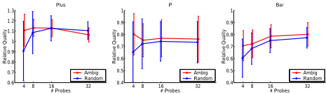
Figure 8: Comparison of influence-based model decomposition quality using random and ambiguity-directed probes, for three different problems: (left) plus; (middle) p; (right) bar. Results are relative to spectral partitioning.

quality q (0 ≤ q ≤ 1) for a partition P of a set of nodes S as follows (i is the influence):

Fig. 8 summarizes the results. The ambiguity-directed method generally does much better than random for a given number of probes, both in mean and standard deviation of quality, and it generally can do as well with 4-8 probes as random sampling can with 16-32. One interesting case is the taper in the plus-shaped piece of material. This is due to over-sampling: the samples are clustered in the middle of the plus, yielding a jagged decomposition that results in a worse quality score. In fact, with default parameters, the ambiguitybased metric declines to add samples beyond about 10, indicating that the field was adequately sampled. In order to achieve the desired number of samples, parameters were set to force sampling for only small information gain.

5 Discussion

The idea of selective sampling to satisfy particular design criteria arises in many contexts, such as Gaussian quadrature, spline smoothing in geometric design, remote sensing data acquisition, crystallography [Gopalakrishnan et al., 2000] and engineering design optimization. In data mining, sampling has been viewed as a methodology to avoid costly disk accesses (this thread of research, however, doesn't address the issue of where to sample) [Kivinen and Mannila, 1994]. All these approaches (including ours) rely on capturing properties of a desirable design in terms of a novel objective function.

The distinguishing feature of our work is that it uses spatial information gleaned from a higher level of abstraction to focus data collection at the field/simulation code layer. While flavors of the consistent labeling problem in mobile vision have this feature, they are more attuned to transferring information across two successive abstraction levels. The applications presented here are novel in that they span and connect arbitrary levels of abstraction, thus suggesting new ways to integrate qualitative and quantitative simulation [Berleant and Kuipers, 1998].

The effectiveness of our approach relies on the trustworthiness of the ambiguity detection mechanism and the ability to act decisively on new information. In both our applications, this was easily achieved by relying on fairly specific qualitative features whose causes are well understood. However, in other applications (e.g. phase portrait exploration for sensitivity analysis of highly non-normal matrices), it is difficult to distinguish between qualitative changes in problem characteristic and numerical error such as roundoff. In such cases, a more detailed modeling of qualitative behavior should be exploited for ambiguity-directed sampling to be successful. In terms of the pocket study, this might require a domainspecific enumeration of the various ways in which pockets (and ambiguities in detecting them) can arise, and a probabilistic model of the elements of a SAL hierarchy using, say, superpositions of Bayesian expectation-maximization terms.

SAL provides a natural framework for exploiting continuity to uncover structures in spatial data; ambiguity-directed sampling focuses SAL's efforts on clarifying those discontinuities that yield multiple, qualitatively-different interpretations. This effort is leading us to explore a completely probabilistic SAL framework. Such a framework should also be able to incorporate information from multiple, perhaps conflicting, SAL hierarchies. This is an emerging frontier in several applications (such as bioinformatics), where diverse experimental methodologies can cause contradictory results at the highest levels of abstraction. Our work provides some encouraging results addressing such grand-challenge problems.

Acknowledgments

Thanks to Layne T. Watson (Virginia Tech) and Feng Zhao (Xerox PARC) for helpful discussions. This work is supported in part by the following grants to Bruce Randall Donald: National Science Foundation grants NSF IIS-9906790, NSF EIA-9901407, NSF EIA-9802068, NSF CDA-9726389, NSF EIA-9818299, NSF CISE/CDA-9805548, NSF IRI9896020, and NSF IRI-9530785, U. S. Department of Justice contract 2000-DT-CX-K001, and an equipment grant from Microsoft Research; and NSF grant EIA-9984317 to Naren Ramakrishnan.