
Reasoning with Cause and Effect
Proceedings of the Sixteenth International Joint Conference on Artificial Intelligence. Awards. Pages 1437-1448.
© 1999 International Joint Conferences on Artificial Intelligence
Abstract
This paper summarizes concepts, principles, and tools that were found useful in applications involving causal modeling. 1 The principles are based on structural-model semantics, in which functional (or counterfactual) relationships, representing autonomous physical processes are the fundamental building blocks. The paper presents the formal basis of this semantics, illustrates its application in simple problems and discusses its ramifications to computational and cognitive problems concerning causation.
- [Balke and Pearl, 1994] A. Balke and J . Pearl. Proba- bilistic evaluation of counterfactual queries. In Pro- ceedings of the Twelfth National Conference on Arti- ficial Intelligence, volume Volume I, pages 230-237.
- [Balke and Pearl, 1995] A. Balke and J. Pearl. Counter- factuals and policy analysis in structural models. In P. Besnard and S. Hanks, editors, Uncertainty in Arti- ficial Intelligence 11, pages 11-18.
- Morgan Kaufmann, San Francisco, 1995.
- [Breese and Heckerman, 1996] J.S. Breese and D. Heck- erman. Decision-theoretic troubleshooting: A frame- work for repair and experiment. In E. Horvitz and F. Jensen, editors, Proceedings of the Twelfth Confer- ence on Uncertainty in Artificial Intelligence, pages 124-132.
- Morgan Kaufmann, San Francisco, CA, 1996.
- [Cartwright, 1989] N. Cartwright. Nature's Capacities and Their Measurement. Clarendon Press, Oxford, 1989.
- [Dawid, 1997] A.P. Dawid. Causal inference without counterfactuals. Technical report, Department of Sta- tistical Science, University College London, UK, 1997.
- [De Kleer and Brown, 1986] J. De Kleer and J.S. Brown. Theories of causal ordering. Artificial Intelli- gence, 29(1):33-62, 1986.
- [Dechter and Pearl, 1991] R. Dechter and J. Pearl. Di- rected constraint networks: A relational framework for casual modeling. In Proceedings of the 12th International Joint Conference of Artificial Intelli- gence (IJCAI-91), pages 1164-1170, Sydney, Aus- tralia, 1991.
- Morgan Kaufmann, San Mateo, CA.
- [Druzdzel and Simon, 1993] M.J. Druzdzel and H.A. Si- mon. Causality in Bayesian belief. In D. Heckerman and A. Mamdani, editors, Proceedings of the Ninth Conference on Uncertainty in Artificial Intelligence, pages 3-11, San Mateo, CA, 1993.
- Morgan Kaufmann. [Eells, 1991]
- E. Eells. Probabilistic Causality. Cam- bridge University Press, Cambridge, MA, 1991.
- [Eshghi and Kowalski, 1989] K. Eshghi and R.A. Kowalski. Abduction compared with negation as falure. In G. Levi and M. Martelli, editors, Proceed- ings of the Sixth International Conference on Logic Programming, pages 234-254. MIT Press, 1989.
- [Fikes and Nilsson, 1971] R.E. Fikes and N.J . Nilsson. STIRPS: A new approach to the application of theo- rem proving to problem solving. Artificial Intelligence, 2(3/4):189-208, 1971.
- [Fine, 1975] K. Fine. Review of lewis' counterfactuals. Mind, 84:451-458, 1975.
- [Fine, 1985] K. Fine. Reasoning with Arbitrary Objects. B. Blackwell, New York, 1985.
- [Fisher, 1970] F.M. Fisher. A correspondence princi- ple for simultaneous equations models. Econometrica, 38(1):73-92, January 1970.
- [Galles and Pearl, 1997] D. Galles and J. Pearl. Axioms of causal relevance. Artificial Intelligence, 97(1-2):9- 43, 1997.
- [Galles and Pearl, 1998] D. Galles and J. Pearl. An axiomatic characterization of causal counterfactuals. Foundation of Science, 3(1):151-182, 1998.
- [Geffner, 1992] H. Geffner. Default Reasoning: Causal and Conditional Theories. MIT Press, Cambridge, MA, 1992.
- [Ginsberg and Smith, 1987] M.L. Ginsberg and D.E. Smith. Reasoning about action I: A possible worlds approach. In Frank M. Brown, editor, The Frame Problem in Artificial Intelligence, pages 233-258.
- Mor- gan Kaufmann, Los Altos, CA, 1987.
- [Ginsberg, 1986] M.L. Ginsberg. Counterfactuals. Arti- ficial Intelligence, 30(35-79), 1986.
- [Good, 1961] I.J. Good. A causal calculus, I. British Journal for the Philosophy of Science, 11:305-318, 1961.
- [Halpern, 1998] J.Y. Halpern. Axiomatizing causal rea- soning. In G.F. Cooper and S. Moral, editors, Uncer- tainty in Artificial Intelligence, pages 202-210.
- Mor- gan Kaufmann, San Francisco, CA, 1998.
- [Heckerman and Shachter, 1995] D. Heckerman and R. Shachter. Decision-theoretic foundations for causal reasoning. Journal of Artificial Intelligence Research, 3:405-430, 1995.
- [Heckerman et al., 1999] D. Heckerman, C. Meek, and G. Cooper. A Bayesian approach to causal discovery. In C. Glymour and G. Cooper, editors, Computation and Causation, pages 143-167. AAAI Press, Menlo Park, CA, 1999.
- [Hume, 1748] D. Hume. An Enquiry Concerning Human Understanding, 1748. Reprinted Open Court Press, LaSalle, 1958.
- [Iwasaki and Simon, 1986] Y. Iwasaki and H.A. Simon. Causality in device behavior. Artificial Intelligence, 29(1):3-32, 1986.
- [Katsuno and Mendelzon, 1991] H. Katsuno and A.O. Mendelzon. On the difference between updating a knowledge base and revising it. In Principles of Knowledge Representation and Reasoning: Proceed- ings of the Second International Conference, pages 387-394, Boston, MA, 1991.
- [Lewis, 1973] D. Lewis. Causation. Journal of Philoso- phy, 70:556-567, 1973.
- [Lewis, 1979] D. Lewis. Counterfactual dependence and time's arrow. Nous, 13:418-446, 1979.
- [Lewis, 1986] D. Lewis. Philosophical Papers, volume II. Oxford University Press, New York, 1986.
- [Lin, 1995] F. Lin. Embracing causality in specifying the indeterminate effects of actions. In Proceedings of the Fourteenth International Joint Conference on Artificial Intelligence (IJCAI-95}, Montreal, Quebec, 1995.
- [McCarthy and Hayes, 1969] J . McCarthy and P. Hayes. Some philosophical problems of artificial intelligence. In B. Meltzer and D. Michie, editors, Machine Intel- ligence, volume Volume 4, pages 463-502. Edinburgh University Press, Edinburgh, 1969.
- [Mill, 1843] J.S. Mill. System of Logic, volume 1.
- John W. Parker, London, 1843.
- [Nayak, 1994] P. Nayak. Causal approximations. Artifi- cial Intelligence, 70:277-334, 1994.
- [Pearl and Verma, 1991] J. Pearl and T . Verma. A the- ory of inferred causation. In J.A. Allen, R. Fikes, and E. Sandewall, editors, Principles of Knowledge Rep- resentation and Reasoning: Proceedings of the Sec- ond International Conference, pages 441-452.
- Morgan Kaufmann, San Mateo, CA, 1991.
- [Pearl, 1988] J. Pearl. Probabilistic Reasoning in Intel- ligent Systems.
- Morgan Kaufmann, San Mateo, CA, 1988.
- [Pearl, 1994] J. Pearl. A probabilistic calculus of actions. In R. Lopez de Mantaras and D. Poole, editors, Un- certainty in Artificial Intelligence 10, pages 454-462.
- Morgan Kaufmann, San Mateo, CA, 1994. [Pearl, 1995]
- J. Pearl. Causal diagrams for experimental research. Biometrika, 82:669-710, December 1995.
- [Pearl, 1996] J. Pearl. Structural and probabilistic causality. In D.R. Shanks, K.J. Holyoak, and D.L. Medin, editors, The Psychology of Learning and Mo- tivation, volume 34, pages 393-435. Academic Press, San Diego, CA, 1996.
- [Pearl, 1999a] J. Pearl. Causality, 1999. Forthcoming.
- [Pearl, 1999b] J. Pearl. Probabilities of causation: Three counterfactual interpretations and their identi- fication. Technical Report R-261, Department of Com- puter Science, University of California, Los Angeles, CA, 1999. Forthcoming, Synthese.
- [Poole, 1985] D. Poole. On the comparison of theories: Preferring the most specific explanations. In Proceed- ings of International Conference on Artificial Intelli- gence (IJCAI-85}, pages 144-147, Los Angeles, CA, 1985.
- [Reiter, 1987] R. Reiter. A theory of diagnosis from first principles. Artificial Intelligence, 32(1):57-95, 1987.
- [Robins, 1986] J.M. Robins. A new approach to causal inference in mortality studies with a sustained expo- sure period -applications to control of the healthy workers survivor effect. Mathematical Modeling, 7:1393-1512, 1986.
- [Sandewall, 1994] E. Sandewall. Features and Fluents, volume 1. Clarendon Press, Oxford, 1994.
- [Serrano and Gossard, 1987] D. Serrano and D.C. Gos- sard. Constraint management in conceptual design. In D. Sriram and R.A. Adey, editors, Knowledge Based Expert Systems in Engineering: Planning and De- sign, pages 211-224. Computational Mechanics Pub- lications, 1987.
- [Simon and Rescher, 1966] H.A. Simon and N. Rescher. Cause and counterfactual. Philosophy and Science, 33:323-340, 1966.
- [Simon, 1953] H.A. Simon. Causal ordering and identifi- ability. In Wm. C. Hood and T.C. Koopmans, editors, Studies in Econometric Method, pages 49-74. Wiley and Sons, Inc., 1953.
- [Spirtes et al., 1993] P. Spirtes, C. Glymour, and R. Scheines. Causation, Prediction, and Search. Springer-Verlag, New York, 1993.
- [Strotz and Wold, 1960] R.H. Strotz and H.O.A. Wold. Recursive versus nonrecursive systems: An attempt at synthesis. Econometrica, 28:417-427, 1960.
- [Winslett, 1988] M. Winslett. Reasoning about action using a possible worlds approach. In Proceedings of the Seventh American Association for Artificial Intel- ligence Conference, pages 89-93, 1988.
- [Woodward, 1997] J. Woodward. Explanation, in- variance and intervention. Philosophy of Science, 64(S):26-S41, 1997.
References were extracted automatically from the PDF and may contain errors.
Full text extracted automatically from the PDF; figures, tables and equations may differ. The PDF is the version of record.
1 Introduction
The central theme in this paper is the interpretation of causality as a computational scheme devised to identify invariant relationships in a domain, so as to facilitate prediction of the effects of actions. This conception h~ been a guiding paradigm to several research commum ties in (and outside) AI, most notably those connected with causal discovery, troubleshooting, policy making, planning under uncertainty, modeling behavior of phys ical systems, and theories of action and change. How ever, the languages and technicalities developed in the~e diverse areas often tend· to obscure their common bas1c principles and thus discourage the transfer of ideas across disciplines. The purpose of this paper is to explicate common principles in simple and familiar mathemati cal form, using little more than propositional calculus, to encourage broader and more effective usage of causal modeling in AI and its peripheries.
After casting the concepts of "causal model," "ac tions " and "counterfactuals" in mathematical terms we will demonstrate by examples how counterfactual ques tions can be answered from both deterministic and prob abilistic causal models (Section 3). In Section 4, I will argue that planning and decision making are exercises in counterfactual reasoning. This will set the stage for Sec tion 4.1, where I discuss the empirical content of coun terfactuals in terms of policy predictions. Section 4.2 demonstrates the role of counterfactuals in the interpre tation and generation of causal explanations, while Sec tion 4.3 relates the properties of structural models to the task of learning causal relationships from data. We end with discussions of how causal relationships emerge from actions and mechanisms (Section 4.4) and how causal di rectionality can be induced by a set of symmetric equa tions (Section 4.5).
1 Additional background material can be found in the technical papers section of http:/ /bayes.cs.ucla.edu/jp..home.html and will soon appear in book form [Pearl, 1999a].
2 Causes and Counterfactuals
In one of his most quoted passages, David Hume (1748) ties together two aspects of causation: 1. regularity of succession and 2. counterfactual dependency:
"we may define a cause to be an object followed by another, and where all the objects, similar to the first, are followed by object similar to the second, Or , in other words, where, if the first object had not been, the second never had existed" [Hume, 17 48, Section VII].
This passage is puzzling; how can convoluted expressions of the type "if the first object had not been, the second never had existed" illuminate simple commonplace ex pressions like "A caused B"?
The idea of reducing causality to counterfactuals is further echoed by Johri Stuart Mill (1843), and has reached its fruition in the works of David Lewis (1973, 1986). Implicit in this proposal lies an intriguing claim that . counterfactual expressions are less ambiguous to our mind than causal expressions. Although discern ing the truth of counterfactuals requires the generation and examination of possible alternative to the actual situation-a mental task of non-negligible proportions Hume, Mill, and Lewis apparently believed that going through this mental exercise is, nevertheless, simpler than intuiting directly on whether it was A that caused B. How? What mental representation allows humans to process counterfactuals so swiftly and reliably, and what logic governs that process so as to maintain uni form standards of coherence and plausibility?
Structure vs. similarity
According to Lewis' account (1973) , the evaluation of counterfactuals involves the notion of similarity: one or ders possible worlds by some measure of similarity, and the a counterfactual AD-t B (read: "B if it were A" ) is declared true in a world w just in case B is true in all the closest A-worlds to w. 2
This semantics still leaves the question of represen tation unsettled: 1. What choice of similarity measure would make counterfactual reasoning compatible with ordinary conception of cause and effect? 2. What men tal representation of worlds ordering would render the computation of counterfactuals manageable and practi cal in man and machine.
In his initial proposal, Lewis was careful to keep his formalism general, and, save for the requirement that every world be closest to itself, he did not impose any structure on the similarity measure. However, plausible sentences such as: "Had Nixon pressed the button, a nu clear war would have started," [Fine, 1975]. tells us im mediately that similarity of appearance is inadequate-a world in which the button happened to be disconnected would be many times more similar to our world than the one yielding a nuclear blast. Thus, similarity mea sures must respect our conception of causallaws. 3 Lewis (1979) has subsequently set up an intricate system of weights and priorities among various dimensions of simi larity: size of "miracles" (violations oflaws), matching of facts, temporal precedence etc., to bring similarity closer to causal intuition. But these priorities turned out rather post-hoc (reminiscent of priorities in nonmonotonic log ics) and still lead to counterintuitive inferences. The structural account, to be described next , escapes these problems by avoiding similarities altogether, and defin ing counterfactuals directly on causallaws. 4
3 Structural Model Semantics
We start with a definition of deterministic "causal model," which consists of functional relationships among variables of interest, each relationship representing an autonomous mechanism. Causal and counterfactuals re lationships are then defined in terms of response to lo cal modifications of those mechanisms. Probabilistic re lationships emerge by assigning probabilities to back ground conditions.
2 Related possible-world semantics were introduced in ar tificial intelligence to represent actions and database updates [Ginsberg, 1986; Ginsberg and Smith, 1987; Winslett, 1988; Katsuno and Mendelzon, 1991] .
3 In this respect, Lewis' reduction of causes to counterfac tuals is somewhat circular.
4 This account builds on Balke and Pearl (1994, 1995), Galles and Pearl {1997, 1998) , and Halpern (1998) . Related approaches have been proposed in Simon and Rescher (1966) and Robins (1986) .
3.1 Definitions: Causal models, actions and counterfactuals
In standard logics, a model is a mathematical object that assigns truth values to sentences in a well formed language. A causal model, naturally, should encode the truth values of sentences that deal with causal relation ships, these include action sentences (e.g., "A will be true if we do B," counterfactuals (e.g., "A would have been different
if it were not forB") and plain causal utterances (e.g., "A was the cause of B" or "B occurred despite of A") .
Definition 3.1 (Causal mode0
A causal model is a triple
where
- ( i) U is a set of background variables, (also called exogenous), that are determined by factors outside the model.
- ( ii) V is a set {V1 , V2, ... , Vn} of variables, called en dogenous, that are determined by variables in the model, namely, variables in U U V.
- (iii) F is a set of functions {h, /2, ... , fn} where each /i is a mapping from UU(V\ Vi) to Vi. In other words, each f i tells us the value of Vi given the values of all other variables in U U V. Symbolically, the set of equations F can be represented by writing
where pai is any realization of the unique minimal set of variables P Ai in V /Vi (connoting parents) that renders /i nontrivial. Likewise, Ui ~ U stands for the unique minimal set of variables in U that renders /i nontrivial.
Every causal model M can be associated with a causal diagram, that is, a directed graph, G(M), in which each node corresponds to a variable in V and the directed edges point from members of P Ai toward Vi.
Definition 3.2 (Submode0
Let M be a causal model, X be a set of variables in V, and x be a particular realization of X. A submodel Mx of M is the causal model
where
In words, Fx is formed by deleting from F all functions fi corresponding to members of set X and replacing them with the set of constant functions X = x.
Submodels are useful for representing the effect of lo cal actions and hypothetical changes, including those dictated by counterfactual antecedents. If we interpret each function /i in F as an independent physical mech anism and define the action do( X = x) as the minimal change in M required to make X = x hold true under any u, then Mx represents the model that results from such a minimal change, since it differs from M by only those mechanisms that directly determine the variables in X. The transformation from M to Mx modifies the algebraic content ofF, which is the reason for the name modifiable structural equations used in [Galles and Pearl, 1998).5
Definition 3.3 (Effect of action)
Let M be a causal model, X be a set of variables in V, and x be a particular realization of X. The effect of action do(X = x) on M is given by the submodel Mx.
Definition 3.4 (Potential response)
Let Y be a variable in V, and let X be a subset of V. The potential response of Y to action do(X = x), denoted Yx ( u), is the solution for Y of the set of equations Fx. 6
We will confine our attention to actions in the form of do(X = x). Conditional actions, of the form "do(X = x) if Z = z" can be formalized using the replacement of equations by functions of Z, rather than by constants [Pearl, 1994]. We will not consider disjunctive actions, of the form "do(X = x or X= x')," since these complicate the probabilistic treatment of counterfactuals.
Definition 3.5 ( CounterfactuaQ
Let Y be a variable in V, and let X a subset of V. The counter-factual sentence "The value that Y would have obtained, had X been x" is interpreted as denoting the potential response Yx ( u).
Definition 3.5 thus interprets the counterfactual phrase "had X been x" in terms of a hypothetical exter nal action that modifies the actual course of history and enforces the condition "X = x" with minimal change of mechanisms. This is a crucial step in the semantics of counterfactuals [Balke and Pearl, 1994], as it permits x to differ from the current value of X(u) without cre ating logical contradiction; it also suppresses abductive inferences (or backtracking) from the counterfactual an tecedent X = x. 7
Definition 3.6 (Probabilistic causal modeQ
A probabilistic causal model is a pair
5 Structural modifications date back to Simon (1953), and is also used in McCarthy and Hayes (1969). An explicit trans lation of interventions into "wiping out" equations from the model was first proposed by Strotz and Wold (1960) and later used in Fisher (1970), Spirtes et al. (1993), and Pearl (1995) . A similar notion of sub-model is introduced in Fine (1985), though not specifically for representing actions and counterfactuals.
6 Galles and Pearl (1998) required that Fx has a unique solution, a requirement later relaxed by Halpern (1998) . Uniqueness of solution is ensured in recursive systems, i.e., where G(M) is a cyclic.
7 Simon and Rescher (1966, p. 339) did not include this step in their definition of counterfactuals and ran into dif ficulties with unwarranted backward inferences triggered by the antecedents.
where M is a causal model and P(u) is a probability function defined over the domain of U.
P(u), together with the fact that each endogenous variable is a function of U, defines a probability distri bution over the endogenous variables. That is, for every set of variables Y ~ V, we have
The probability of counterfactual statements is defined in the same manner, through the function Yx(u) induced by the submodel Mx:
Likewise a causal model defines a joint distribution on counterfactual statements, i.e., P(Yx = y, Zw = z) is defined for any sets of variables Y, X, Z, W, not nec essarily disjoint. In particular, P(Yx = y, X = x') and P(Yx = y, Yx' = y') are well defined for x =f. x', and are given by
and
When x and x' are incompatible, Yx and Yx' cannot be measured simultaneously, and it may seem meaning less to attribute probability to the joint statement "Y would be y if X = x and Y would be y' if X = x"' [Dawid, 1997]. The definition of Yx and Yx' in terms of two distinct submodels, driven by a standard probability space over U, provides a simple interpretation of prob abilities of counterfactuals and further illustrates that such probabilities can be encoded rather parsimoniously using P(u) and F.
Of particular interest to us would be probabilities of counterfactuals conditional on actual observations. For example, the probability that event X = x "was the cause" of event Y = y may be interpreted as the prob ability that Y would not be equal to y had X not been x, given that X = x and Y = y have in fact occurred (Pearl, 1999b). Such probabilities require the evaluation of expressions of the form P(Yx' = y'IX = x, Y = y) with x' and y' incompatible with x and y, respectively. Eq. ( 4) allows the evaluation of this quantity using a 3-step procedure that we summarize in a theorem.
Theorem 3. 7 Given model < M, P(u) >, the condi tional probability P(BAie) of a counter-factual sentence "If it were A then B, " given evidence e, can be evalu ated using the following three steps:
1. Abduction- update P(u) by the evidence e, to ob tain P(ule).
- Action-Modify M by the action do(A), where A is the antecedent of the counter/actual, to obtain the submodel MA.
- Prediction-Use the modified model < MA,P(uie) > to compute the probability of B, the consequence of the counter/actual.
In temporal metaphors, this 3-step procedure amounts to (1) explaining the past (U) in light of the current evidence e, (2) bending the course of history (minimally) to comply with the hypothetical condition X = x and, finally, (3) predicting the future (Y) on the basis of (1) and (2).
3.2 Evaluating counterfactuals: Deterministic analysis
Example-1, The firing squad
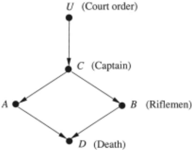
Consider a 2-man firing squad as depicted in Fig. 1, where A, B, C, D and U stand for the following proposi tions:
U Court orders the execution
C = Captain gives a signal
A Rifleman-A shoots ·
B = Rifleman-B shoots
D Prisoner dies
Assume that the court's decision is unknown, that both riflemen are accurate, alert and law abiding, and that the prisoner is not likely to die from fright or other extraneous causes. We wish to construct a formal rep resentation of the story, so that the following sentences can be evaluated mechanically:
- Sl. (prediction): If rifleman-A did not shoot, the pris oner is alive. Formally, ·A => ·D
- S2. (abduction): If the prisoner is alive, then the Cap tain did not signal. Formally, ·D => ·C
- S3. (transduction): If rifleman-A shot, then B shot as well. Formally, A=> B
- S4. (action): If the captain gave no signal and rifleman A decides to shoot, the prisoner will die and B will not shoot. Formally, ·C => D A & ·B A
- S5. (counterfactua0: If the prisoner is dead, then even if A were not to have shot, the prisoner would still be dead. Formally, D => D~A
Evaluating standard sentences
To prove the first three sentences we need not invoke causal models; these involve standard logical connectives and can be handled by standard logical inference. The story can be captured in any convenient logical theory, T , for example,
and the validity of S1-S3 can easily be verified by deriva tion from T.
Note, however, that the two-way implications in Tare necessary for supporting abduction; if we were to use one-way implications, e.g., C =>A, we would not be able to conclude C from A. In standard logic, this symme try removes all distinctions among prediction (reasoning forward in time), abduction (reasoning from evidence to explanation) and transduction (reasoning from evidence to explanation, then from explanation to predictions). In non-standard logics (e.g., logic programming), were the implication sign dictates the direction of inference and even contraposition is not supported, special ma chinery must be invoked to perform abduction [Eshghi and Kowalski, 1989). Note also that the feature which renders S1-S3 manageable in standard logic is that they all deal with epistemic inference, that is, inference from beliefs to beliefs about a static world.
Evaluating action sentences
Sentence S4 invokes a deliberate action and, from (Defi nition 3.3) it must violate some premises, or mechanisms, in the initial theory. To formally identify what remains invariant under the action, we must incorporate causal relationships into the theory. One symbolic representa tion of the causal model corresponding to our story is as follows:
Model M:
C = U
(U)
(C)
Here we use equality, rather than implication signs, first, to permit two-way inference and, second, to stress the fact that each equation represents an autonomous mechanism, (an "integrity-constraint" in the language of databases); it remains invariant unless specifically vi olated. We further use parenthetical symbols next to each equation, to explicitly identify the dependent vari able (on the left hand side) in the equation, thus rep resenting the causal directionality associated with the arrows in Fig. 1.
To evaluate S4, we follow Definition 3.3 and form the submodel MA, in which the equation A= Cis replaced by A (simulating the decision of of rifleman-A to shoot regardless of signals), and obtain
Facts: ·C
Conclusions: A, D, ·B, ·U, ·C
We see that, given the fact ·C, we can easily deduce D and ·B and thus confirm the validity of S4.
It is important to note that "problematic" sentences like S4, whose antecedent violates one of the basic premises in the story (i.e., that both riflemen are law abiding) are handled naturally within the same deter ministic setting in which the story is told. Alternative approaches would be to insist on re-formulating the prob lem probabilistically (see next subsection) or on using an ab predicate, so as to tolerate exceptions to the law A = C. Such reformulations are unnecessary; the struc tural approach permits us to draw the intended infer ences in the natural, deterministic formulation of the story.
Evaluating counterfactuals
To evaluate the counterfactual sentence S5, we can fol low the steps of Theorem 3.7, though no probabilities are involved. We first add the fact D to the original model, M, evaluate U, then form the submodel M~A and, finally, re-evaluate the truth of D in M~A, using the value of U found in the first step. These steps can be combined into one, noting that the value of U is the only information that is carried over from Step-1 to Step2; all other propositions must be re-evaluated subject to the new modification of the model.
If we distinguish post-modification variables from pre modification variables by a star, we can combine M and M~A into one logical theory and prove the validity of S5 by purely logical inference in the combined theory. To illustrate, we write S5 as D => D:A. (read: If D is true in the actual world, then D would also be true in the hypothetical world created by the modification ·A*) and prove the validity of D* in the combined theory:
Combined Theory:
| (U) | |
|---|---|
| C* =U | C=U (C) |
| •A* | A=C (A) |
| B* = C* | B=C (B) |
| D* =A* v B* | D=AVB (D) |
Facts: D
Conclusions: U, A, B, C, D, ·A*, C*, B*, D*
Note that U is not starred, reflecting the assumptions that background conditions remain unaltered, thus serv ing as carriers of persistence information between the actual world to the hypothetical world.
It is worth reflecting at this point on the difference between S4 and S5. Syntactically, the two appear to be identical and, yet, we labeled S4 an "action" sen tence and S5 a "counterfactual" sentence. The differ ence lies in the relationship between the given fact and the antecedent of the counterfactual (i.e., the "action" part). In S4 the fact given (C) is not affected by the antecedent (A) while in S4, the fact given (D) is poten tially affected by the antecedent (·A). The difference between these two situations is fundamental, as can be seen from their methods of evaluation. In evaluating S4, we knew in advance that C would not be affected by the model modification do(A) and, therefore, we were able to add C directly to the modified model MA. In eval uating S5, on the other hand, we were contemplating a possible reversal, from D to ·D, due to the modifica tion do( ·A) and, therefore, we had to first add fact D to the pre-action model M, summarize its impact via U, and reevaluate D once the modification do( ·A) takes place. Thus, although the causal effect of actions can be expressed syntactically as a counterfactual sentence, this need to route the impact of known facts through U makes counterfactuals a different species than actions.
We should also emphasize that most counterfactuals utterances in natural language presume knowledge of facts that are affected by the antecedent. When we say, for example, "B would be different if it were not for A," we imply knowledge of what the actual value of B is and that B is susceptible to A. It is this sort of sentences that gives counterfactuals their unique character, distinct of action sentences. 8
3.3 Evaluating counterfactuals: Probabilistic analysis
Assume the following modification of the story:
- There is a probability P(u = 1) = p that the court has ordered the execution.
- Rifleman-A has a probability q of pulling the trigger out of nervousness (w=1).
8 Balke and Pearl (1994) also noted that this sort of sen tences a require a more detailed specifications for their eval uation; some knowledge of the functional mechanisms {!;} is necessary. See also [Heckerman and Shachter, 1995].
3. Rifleman-A nervousness is independent of U.
With these assumptions, we wish to compute the prob ability P(....,D~AID) that the prisoner would be alive if A were not to have shot, given that the prisoner is in fact dead.
Following Theorem 3.7, our first step (abduction) is to compute the posterior probability P(u, wiD), where U and W are the two background variables involved.
The second step (action) is to form the submodel:
The last step (prediction) is to compute P( -,D) in the probabilistic model above. Noting that ....,D = ....,u, the expected result follows:
3.4 The twin-network method
A major practical difficulty in the procedure described above is the need to compute, store and use the posterior distribution P(ule) , where u stand for the set of all back ground variables in the model. As is illustrated in the last example, even when we start with a model in which the background variables are mutually independent, con ditioning on e normally destroys this independence, and makes it necessary to carry over a full description of the joint distribution of U, conditional on e; such description may be prohibitively large.
A graphical method of overcoming this difficulty is de scribed in Balke and Pearl (1994), which uses two net works, one to represent the actual world, and one to represent the hypothetical world (Fig. 2) .
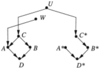
The two networks are identical in structure, save for the arrows entering A, which have been deleted to mir ror the equation deleted from M~A· Like Siamese twins, the two networks share the background variables (in our case U and W) since those remain invariant under modi fication. The endogenous variables are replicated and la beled distinctly, because they may obtain different values in the hypothetical vis a vis the actual world. The task of computing P(-,D) in the model< MA,P(u,viD) > thus reduces to that of computing P( ....,D*ID) in the twin network shown. Such computation can be performed by standard evidence-propagation techniques in a Bayesian network-the distribution P(ule) need not be explicated, conditional independencies can be exploited, and local computation methods can be employed such as those summarized in many textbooks (e.g., [Pearl, 1988]).
The twin-network representation also offers a use ful way of testing independencies among counterfactual quantities. To illustrate, suppose we wish to test whether BA is independent of D, given C. This can be verified by noting that C d-separates D from B* in the twin network shown in Fig. 2.
The verification of such independencies is important for deciding if the ramifications of certain plans can be inferred from statistical data, because these independen cies permit us to reduce counterfactual probabilities to ordinary probabilistic expression on observed variables (Pearl, 1995; Galles and Pearl, 1998].
4 Applications and Interpretation of Structural Models
Computing counterfactual probabilities is not an aca demic exercise; it represents in fact the typical case in almost every decision making situation. Whenever we undertake to predict the effect of policy, two consider ations apply. First, the policy variables (e.g., interest rates in economics, pressure and temperature in process control) are rarely exogenous. Policy variables are en dogenous when we observe a system under operation and turn exogenous in the planning phase, when we contem plate actions and changes. Second, policies are rarely evaluated in the abstract; rather, they are brought into focus by certain eventualities that demand remedial cor rection. In troubleshooting, for example, we observe un desirable effects e that are influenced by other conditions X = x and wish to predict whether an action that brings about a change in X would remedy the situation. These are precisely the three steps that Theorem 3. 7 attaches to the evaluation of counterfactuals, and have been applied indeed to the evaluation of economic policies [Balke and Pearl, 1995] and to repair-test strategies in troublesho.ot ing [Breese and Heckerman, 1996]. The reasons for usmg hypothetical phrases in practical decision-making situa tions is discussed in the next section.
4.1 The empirical content of counterfactuals
Consider Ohm's law V =JR. The empirical content of this law can be encoded in two alternative forms.
- Predictive form: If at time t0 we measure current Io and voltage Vo then, ceteras paribum, at any fu ture times t > to, if the current flow will be I(t) the voltage drop will be:
- Counterfactual form: If at time t 0 we measure current Io and voltage Vo then, had the current flow at time to been I', instead of !0 , the voltage drop would have been:
On the surface, it seems that the predictive form makes meaningful and testable empirical claims while the counterfactual form merely speculates about events that have not, and could not have occurred; as it is im possible to apply two different currents into the same resistor at the same time. However, if we interpret the counterfactual form to mean no more nor less than a con versational short hand of the predictive form, the empir ical content of the former shines through clearly. Both enable us to make an infinite number of predictions from just one measurement (!0 , V0 ), and both derive their va lidity from a scientific law (Ohm's law) which ascribes a time-invariant property (the ratio V /I) to any physical object.
But if counterfactual statements are merely a round about way of stating sets of predictions, why do we re sort to such convoluted modes of expression instead of using the predictive mode directly? One obvious an swer is that we often use counterfactuals to convey, not the predictions themselves, but the logical consequences of those predictions. For ·example, the intent of saying: "if A were not to have shot, the prisoner would still be alive" may be merely to convey the factual information that B did not shoot. The counterfactual mood, in this case, serves to supplement the fact conveyed with logical justification based on a general law. The less obvious an swer rests with the qualification "ceteras paribum" that accompanies the predictive claim, which is not entirely free of ambiguities. What should be held constant when we change the current in a resistor? The temperature? the laboratory equipments? the time of day? Certainly not the reading on the voltmeter? Such matters must be carefully specified when we pronounce predictive claims and take them seriously. Many of these specifications are implicit (hence superfluous) when we use counter factual expressions, especially when we agree over the underlying causal model. For example, we do not need to specify under what temperature and pressure future predictions should hold true; these are implied by the statement "had the current flow at time to been I', in stead of Io." In other words, we are referring to precisely those conditions that prevailed in our laboratory at time to. That statement also implies that we do not really mean for anyone to hold the reading on the voltmeter constant-variables should run their natural course and the only change we should envision is in the mechanism which, according to our causal model, is currently deter mining the current.
To summarize, a counterfactual statement might well be interpreted to convey a set of predictions under well defined set of conditions, those prevailing in the factual part of the statement. For these predictions to be valid, two components must remain invariants: the laws (or mechanisms) and the boundary conditions. Cast in the language of structural models, the laws correspond to the equations {h} and the boundary conditions correspond to the state of the background variables U. Thus, a pre condition for the validity of the predictive interpretation of a counterfactual statement is the assumption that U will remain the same at the time where our predictive claim is to be applied or tested.
This is best illustrated using a betting example. We must bet heads or tails on the outcome of a fair coin toss; we win a dollar if we guess correctly, lose if we don't. Suppose we bet heads and we win a dollar, with out glancing at the outcome of the coin. Consider the counterfactual "Had I bet differently I would have lost a dollar." The predictive interpretation of this sentence translates into the implausible claim: "If my next bet is tails, I will lose a dollar." For this claim to be valid, two invariants must be assumed: the payoff policy and the outcome of the coin. While the former is a plausi ble assumption in betting context, the latter would be realized in only rare circumstances. It is for this reason that the predictive utility of the statement "Had I bet differently I would have lost a dollar" is rather low, and some would even regard it as hind-sighted nonsense. It is the persistence across time of U and f(x, u) that en dows counterfactual expressions with predictive power; take this persistence away, and the counterfactual loses its obvious economical utility.
However, there is an element of utility in counterfac tuals that does not translate immediately to predictive payoff, and may explain, nevertheless, the ubiquity of counterfactuals in human discourse. I am thinking of explanatory value. Suppose, in the betting story, coins were tossed afresh for every bet. Is there no value what soever to the statement "Had I bet differently I would have lost a dollar?" I believe there is; it tells us that we are not dealing here with a whimsical bookie, but one who at least glances at the bet, compares it to some standard, and decides a win or a loss using a consistent policy. This information may not be very useful to us as players, but it may be useful to say state inspectors who come every so often to calibrate the gambling machines to ensure the State's take of the profit. More signifi cantly, it may be useful to us players, too, if we venture to cheat slightly, say by manipulating the trajectory of the coin, or by installing a tiny transmitter to tell us which way the coin landed. For such cheating to work, we should know the policy y = f(x , u) and the state ment "Had I bet differently I would have lost a dollar?" reveals important aspects of that policy.
Is it far fetched to argue for the merit of counterfac tuals by hypothesizing unlikely situations where players cheat and rules are broken? I suggest that such un likely operations are precisely the norm for gauging the explanatory value of sentences. It is the nature of any causal explanation that its utility be amortized not over standard situations but, rather, over novel settings which require innovative manipulations of the standards. The utility of understanding how TV works comes not from turning the knobs correctly, but from the ability to re pair a TV set when it breaks down. Recall that every causal model advertises, not one, but a host of submod els, each created by violating some laws. The autonomy of the mechanisms in a causal model stands therefore for an open invitation to remove or replace those mecha nisms, and it is only natural that the explanatory value of sentences be judged by how well they predict the ram ifications of such replacements.
4.2 Causal explanations, utterances, and their interpretation
It is commonplace wisdom that explanation improve un derstanding, and that he who understands more, can reason and learn more effectively. It is also generally ac cepted that the notion of explanation cannot be divorced from that of causation; e.g., a symptom may explain our belief in a disease, but it does not explain the disease itself. However, the precise relationship between causes and explanations is still a topic of much discussion in philosophy [Woodward, 1997]. Having a formal theory of counterfactuals, in both deterministic and probabilis tic settings, casts new light on the question explanation adequacy, and opens new possibilities for automatic gen eration of explanations by machine.
These possibilities trigger an important basic question: Is explanation a concept based on general causes (e.g., "Drinking hemlock causes death,") or singular causes (e.g., "Socrates' drinking hemlock caused his death,") . action-effect expressions, P(yjdo(x)) ~ P(Yx = y), be long to the first category while counterfactual expres sions, P(Yx' = y'jx, y) belong to the second, since condi tioning on x and y narrows down world scenarios to those compatible with all the specific information at hand.
The classification of causal statements into general and singular categories has been the subject of intensive research in philosophy e.g., see [Good, 1961; Cartwright, 1989; Eells, 1991]. This research has attracted little attention in cognitive science and artificial intelligence, partly because it has not entailed practical inferential procedures, and partly because it was based on prob lematic probabilistic semantics (see Pearl (1996) for dis cussion of probabilistic causality). In the context of machine generated explanations, this classification assumes both cognitive and computational significance. The analysis of counterfactual probabilities [Balke and Pearl, 1994] has uncovered a sharp demarcation line be tween two types of causal queries, those that are an swerable from the pair < P(M), G(M) > (where P(M) is the probability induced by M), and those that require additional information in the form of functional spec ification. Generic causal statements (e.g., P(yjdo(x))) often fall in the first category while counterfactual ex pressions (e.g., P(Yx' = yjx,y)) fall in the second, thus demanding more detailed specifications and higher com putational resources.
The proper classification of explanation into a gen eral or singular category depends on whether the cause x attains its explanatory power relative to its effect y by virtue of x's general tendency to produce y (as com pared with the weaker tendencies of x's alternatives) or by virtue of x being necessary for triggering the chain of events leading to y in the specific situation at hand (as characterized by y and perhaps other facts and observa tions.)
If we base explanations solely on generic tendencies we lose important specific information. For instance, aiming a gun at and shooting a person from 1000 meters away will not qualify as an explanation for that person's death, due to the very low tendency of typical shots fired from such long distances to hit their marks. The fact that spe cial conditions helped the shot hit its mark on that singu lar day will not enter into consideration. If, on the other hand, we base explanations solely on singular-event con siderations then various background factors which are normally present in the world would awkwardly qualify as explanations. The presence of oxygen in the room would qualify as an explanation for the fire that broke out. Clearly, some balance must be made between the necessary and the sufficient, singular and generic compo nents of causal explanation. Basic relationships between these components are explicated in [Pearl, 1999b], using probabilities of counterfactuals.
The following list, taken from [Galles and Pearl, 1997], provides brief examples of utterances used in explana tory discourse and their associated structural-model se mantics. (The necessary aspect of causation is taken as a norm.)
- "X is a cause of Y," if there exist two values x and x' of X and a value u of U such that Yx(u) =J Yx' (u).
- "X is a cause of Y in context Z = z," if there exist two values x and x' of X and a value u of U such that Yxz =J Yx'z(u).
- "X is a direct cause of Y ," if there exist two values x and x' of X, and a value u of U such that Yxr(u) =J Yx'r(u) where r is some realization of V\X.
- "X is an indirect cause of Y ," if X is a cause of Y , and X is not a direct cause of Y.
- "Event X = x may have caused Y = y" if (i) X= x andY= y are true, and
- (ii) There exists a value u of U such that X(u) = x, Y(u) = y, Yx(u) = y and Yx' (u) "1- y for some x' "1- x.
- "The unobserved event X = x is a likely cause of y = y" if
- (i) Y = y is true, and
- (ii) P(Yx = y, Yx' "1- yjY = y) is high for some x' "1- x
- "Event Y = y occurred despite X= x," if
- (i) X= x and Y =yare true, and
- (ii) P(Yx = y) is low.
The preceding list demonstrates the flexibility of mod ifiable structural models in formalizing nuances of causal expressions. Additional nuances, invoking notions such as enabling, preventing, maintaining, and producing, are analyzed in [Pearl, 1999a].
4.3 Structural models, causal discovery and knowledge mining
It is by now fairly well understood that the central aim of the enterprise known as "knowledge discovery" is the identification of invariant (often causal) relation ships in data. What is perhaps less generally appreci ated is that the dual character of causal mechanisms, invariance and autonomy, is the key for the operation of knowledge discovery programs, especially those based on causal graphs.
The invariance property assures us that when one mechanism undergoes change, the others remain intact. Identifying such mechanisms would amount therefore to the acquisition of "knowledge," as it permits us to trans port patterns of behavior from one context to another. The feature of "comprehensibility" or "making sense," which normally accompanies the discovery of knowledge like relationships, is a byproduct of transportability. The autonomy property further tells us what varies from one context to another, and thus provides the clues for identifying those features of the observed data that are context-independent.
One such feature is the so called causal Markov con dition [Spirtes et al., 1993]. It states that, for a causal model to be considered complete, each variable Vi must be independent on all its non-descendants, given its par ents P Ai in G. This parent-screening condition has been the defining feature of Bayesian networks, and has served as the key for many causal discovery algorithms (e.g., [Pearl and Verma,1991; Spirtes etal., 1993]. The rea son that the Markov condition is so often regarded as an inherent feature of causal models rests, again, on the property of in variance, as can be seen from the following theorem.
Theorem 4.1 (causal Markov condition)
Every causal model M for which G(M) is acyclic and in which the ui 's are mutually independent induces a distri
bution P( v1 , · . . , vn) that satisfies the Markov condition relative the causal diagram G(M). [Pearl and Verma, 1991]: 9
This theorem states that the independencies dictated by the Markov condition are invariant to the functional form of fi and to the distributional properties of P(ui)· This invariance renders Markovian independencies reli able clues for inferring the structures of causal models from data; any structure whose Markovian independen cies turn incompatible with the data can safely be ruled out from consideration. The property of autonomy fur ther implies that, as contexts change, accidental inde pendencies are destroyed and only independencies dic tated by the Markov condition are preserved. This pro vides the theoretical basis for the assumption of "stabil ity" [Pearl and Verma, 1991] or "faithfulness" [Spirtes et al., 1993]-the second corner stone in causal discovery algorithms.
Bayesian approaches to causal discovery [Heckerman et al., 1999] also owe their rationale to invariance and autonomy. The assumption of parameter-independence, which is made in all practical Bayesian approaches to model discovery, can be justified only when the parame ters P(viiPai) are attached to stable mechanisms (as op posed to arbitrary conditional probabilities) and when those mechanisms are free to change independently of one another, namely, autonomy.
4.4 From mechanisms to actions to causation
The structural model described in Section 3.1 crystal lizes the conceptual elements behind two highly debated issues in AI, the representation of actions, and the role of causal ordering. We will discuss these problems in turns, since the second builds on the first.
Action, Mechanisms and surgeries
Whether we take the probabilistic paradigm that actions are transformations from probability distributions to probability distributions, or the deterministic paradigm that actions are transformations from states to states, such transformations could in principle be infinitely com plex. Yet, in practice, people teach each other rather quickly what actions normally do to the world, and peo ple predict the consequences of most actions without much hustle. How?
Structural models answer this question by assuming that the actions we normally invoke in common reason ing can be represented as local surgeries. The world consists of a huge number of autonomous and invariant linkages or mechanisms, each corresponding to a physical process that constrains the behavior of a relatively small group of variables. If we understand how the linkages interact with each other (usually they simply share vari ables) we should also be able to predict what the effect of any given action would be: Simply re-specify those few mechanisms that are perturbed by the action, then let the modified assembly of mechanisms interact with one another, and see what state will evolve at equilib rium. If the specification is complete (i.e., M and U are given), a single state will evolve. If the specification is probabilistic (i.e., P(u) is given) a new probability dis tribution will emerge and, if the specification is partial (i.e., some J;'s are not given) a new, partial theory will then be created. In all three cases we should be able to answer queries about post-action states of affair, albeit with decreasing level of precision.
9 Considering its generality and transparency, I would not be surprised if some version of this theorem has appeared earlier in the literature.
The ingredient that makes this scheme operational is the locality of actions. Standing alone, locality is a vague concept because what is local in one space may not be local in another. Structural semantics emphasizes that actions are local in the space of mechanisms and not in the space of variables or sentences or time slots. For ex ample, tipping the left-most object in an array of domino tiles does not appear "local" in physical space, yet it is quite local in the space of mechanisms: Only one mecha nism gets perturbed, that which keeps the left-most tile in erect position; all other mechanisms remain unaltered, as specified, obedient to the usual equations of physics. Locality makes it is easy to specify this action, without enumerating all its ramifications. The listener, assum ing she shares our understanding of domino physics, can figure out for herself the ramifications of this action, or any action of the type: "tip the ith domino tile to the right." Thus, by representing the domain in the form of an assembly of autonomous mechanisms, we have in fact created an oracle capable of predicting the effects of a huge set of actions and action combinations, without us having to explicate those effects.
Laws vs. facts
In order to implement surgical procedures in mechanism space, we need a language in which some sentences are given different status than others; sentences describing mechanisms should be treated differently than those de scribing other facts of life, such as observations, assump tion and conclusions, because the former are presumed stable, while the latter are transitory.
In Bayesian networks, the distinction between laws from facts is made using conditional probabilities. Facts are expressed as ordinary propositions, hence they can obtain probability values and they can be conditioned on; laws, on the other hand, are expressed as conditional probability sentences (e.g., P( accident! careless-driving) = high), hence they should not be assigned probabilities and cannot be conditioned on. A similar distinction has been proposed for nonmonotonic logics by Poole (1985) and Geffner (1992) 10 and a related distinction in the form of domain constraints is used in formal theories of actions (Sandewall 1994; Lin 1995].
10 In database theory, laws are expressed by special sen tences called integrity constraints [Reiter, 1987].
Mechanisms and causal relationships
From our discussion thus far, it may seem that one can construct an effective representation for computing the ramification of actions without appealing to any notion of causation. This is indeed feasible in many areas of physics and engineering. If we have, for instance, a large electric circuit consisting of resistors and voltage sources, and we are interested in computing the effect of chang ing one resistor in the circuit, the notion of causality hardly enters the computation. We simply insert the modified value of the resistor into Ohm's and Kirchoff's equations, and solve the set of (symmetric) equations for the variable needed. This computation can be performed effectively without committing to any directional causal relationship between the currents and voltages.
To understand the role of causality, we should note that, unlike the resistor-network example, most mecha nisms do not have names in common everyday language. We say: "raise taxes," "make him laugh," "press the button," and, in general, do(q) where q is a proposition, not a mechanism. It would be meaningless to say: "in crease this current" or "if this current were higher ... " in the resistor-network example, because there are many (minimal) ways of increasing that current, each gener ating different ramifications. Evidently, commonsense knowledge is not as entangled as resistor networks. In the STRIP language [Fikes and Nilsson, 1971], to use another example, an action is not characterized by the name of the mechanisms it modifies but, rather, by the actions' immediate effects (the ADD and DELETE lists), and these effects are expressed as ordinary propositions. Indeed, if our knowledge is organized causally, this speci fication is sufficient, because each variable is governed by one and only one mechanism (see Definition 3.1). Thus, we should be able to figure out for ourselves which mech anism it is that must be perturbed in realizing the new event, and this should enable us to predict the rest of the scenario.
This important abbreviation defines a new relation among events, a relation we normally call "causation": Event A causes B, if the perturbation needed for real izing A produces the realization of BY Causal abbre viations of this sort are used very effectively for specify ing domain knowledge. Complex descriptions of domain constrains and of how they interact with one another can be summarized in terms of cause-effect relationships be tween events or variables. We say, for example: "If tile i is tipped to the right, it causes tile i + 1 to tip to the right as well"; we do not communicate such knowledge in terms of the tendencies of each domino tile to maintain its physical shape, to respond to gravitational pull and to obey Newtonian mechanics.
11 The word "needed" connotes minimality and can be translated to: " .. .if every minimal perturbation realizing A, produces B". Additional qualifications are discussed in [Pearl, 1999b].
4.5 Simon's causal ordering
Our ability to talk directly in terms of one event caus ing another, (rather than an action altering a mecha nism and the alteration, in turn, producing the effect) is computationally very useful, but, at the same time it requires that the assembly of mechanisms in our domain satisfy certain conditions which accommodate causal di rectionality. Indeed, the formal definition of causal mod els given in Section 3.1 assumes that each equation is designated a distinct privileged variable, situated on its left hand side, that is considered "dependent" or "out put". In general, however, a mechanism may be specified as a functional constraint
without identifying any so called "dependent" variable.
Simon (1953) devised a procedure for deciding whether a collection of such symmetric G functions dictates a unique way of selecting an endogenous "dependent" vari able for each mechanisms (excluding the background variables since they are determined outside the sys tem). Simon asked: when can we order the variables (V1 , V2 , ... , Vn) in such a way that we can solve for each l-'i without solving for any of l-'i 's successors? Such an or dering, if it exists, dictates the direction we attribute to causation. This criterion might at first sound artificial, since the order of solving equations is a matter of com putational convenience while causal directionality is an objective attribute of physical reality. (See [Iwasaki and Simon, 1986], [De Kleer and Brown, 1986], and [Druzdzel and Simon, 1993] for discussion of this issue.) To justify the criterion, let us rephrase Simon's question in terms of actions and mechanism. Assume each mechanism (i.e., equation) can be modified independently of the others and let Ak be the set of actions capable of modifying equation Gk (while leaving other equations unaltered). Imagine that we have chosen an action ak from Ak, and that we have modified G k in such a way that the set of solutions (V1 (u), V2 (u), ... , Vn(u)) to the entire system of equations differs from .what it was prior to the action. If X is the set of endogenous variables constrained by Gk, we can ask which members of X would change by the modification. If only one member of X changes, say Xk, and if the identity of that distinct member remains the same for all choices of ak and u, we designate Xk as the "dependent" variable in G k.
Formally, this property means that changes in ak in duce a functional mapping from the domain of xk to the domain of {V\Xk}; all changes in the system (gen erated by ak) can be attributed to changes in Xk. It would make sense, in such a case, to designate Xk as a "representative" of the mechanism Gk, and we would be justified in replacing the sentence "action ak caused event Y = y" with "Event Xk = Xk caused Y = y" (Y being any variable in the system). The invariance of Xk to the choice of ak is the basis for treating an action as a modality do(Xk = Xk) (Definition 3.3). It provides a license for characterizing an action by its immediate consequence(s), independent of the instrument that ac tually brought about those consequences, and defines in fact the notion of "local action" or "local surgery" .
It can be shown [Nayak, 1994] that the uniqueness of xk can be determined by a simple criterion that involves purely topological properties of the equation set (i.e., how variables are grouped into equations). The criterion is that one should be able to form one-to-one correspon dence between equations and variables and that the cor respondence be unique. This can be decided by solving the matching problem (Serrano and Gossard, 1987] be tween equations and variables. If the matching is unique, then the choice of dependent variable in each equation is unique and the directionality induced by that choice defines a directed acyclic graph (DAG). In Fig. 1, for example, the directionality of the arrows need not be specified externally, they can be determined mechani cally from the set of symmetrical constraints (i.e., logical propositions):
that characterizes the problem. The reader can easily verify that the selection of a privileged variable from each equations is unique and, hence, that the causal di rectionality of the arrows shown in Fig. 1 is inevitable.
Thus, we see that causal directionality, according to Simon, emerges from two assumptions: 1. The partition of variables into background (U) and endogenous (V) sets, and 2. the overall configuration of mechanisms in the model. Accordingly, a variable designated as "de pendent" in a given mechanism may well be labeled "in dependent" when that same mechanism is embedded in a different model. Indeed, the engine causes the wheels to turn when the train goes up hill, and changes role in going down hill.
Of course, if we have no way of determining the back ground variables, then several causal orderings may en sue. In Eq. (7), for example, if we were not given the information that U is a background variable, then ei ther one of {U, A, B, C} can be chosen as background, and each such choice would induce a different ordering on the remaining variables. (Some would conflict with commonsense knowledge,. e.g., that the Captain's sig nal influences the court decision) . The directionality of A -+ D +- B however, would be maintained in all those orderings. The question whether there exists a partition {U, V} of the variables that would yield a causal ordering in a system of symmetric constraints can also be solved (in polynomial time) by topological means [Dechter and Pearl, 1991].
Simon's ordering criterion fails when we are unable to solve the equations one at a time, but must solve a block of k equations simultaneously. In such a case, all the k variables determined by the block would be mu tually unordered, though their relationships with other blocks may still be ordered. This occurs, for example, in economic modeling, which often include feedback loops (e.g., demand affects price and price affects demand). The correspondence between equations and variables, in this case, will not be unique and the directionality of the arrows in the loop would be arbitrary.
In cases where we tend to assert categorically that the flow of causation in a f~edback loop goes clockwise, rather than counterclockwise, the assertion is normally based on the relative magnitudes of forces. For exam ple, turning the faucet would lower the water level in the water tank but there is practically nothing we can do to the water tank that would turn the faucet . When such information is available, causal directionality is deter mined by appealing, again, to the notion of hypothetical intervention and asking whether an external control over one variable in the mechanism necessarily affects the oth ers. This consideration then constitutes the operational semantics for identifying the dependent variables Vi in nonrecursive causal models (Definition 3.1).
The asymmetry that characterizes causal relationships in no way conflicts with the symmetry of physical equa tions. By saying that "X causes Y andY does not cause X" we mean to say that changing a mechanism in which X is normally the dependent variable has a different ef fect on the world than changing a mechanism in which Y is normally the dependent variable. Since two separate mechanisms are involved, the statement stands in perfect harmony with the symmetry we find in the equations of physics.
Acknowledgments
This research was partially supported by grants from NSF, ONR, AFOSR, Microsoft Corporation, and Rock well International.
@inproceedings{ijcai1999p203,
  title     = {Reasoning with Cause and Effect},
  author    = {Pearl, Judea},
  booktitle = {Proceedings of the Sixteenth International Joint Conference on
               Artificial Intelligence, {IJCAI-99}},
  publisher = {International Joint Conferences on Artificial Intelligence},
  editor    = {Thomas Dean},
  pages     = {1437--1448},
  year      = {1999},
  note      = {Awards},
  url       = {https://ijcai.org/proceedings/1999/203},
}
TY - CPAPER TI - Reasoning with Cause and Effect AU - Pearl, Judea T2 - Proceedings of the Sixteenth International Joint Conference on Artificial Intelligence, IJCAI-99 PB - International Joint Conferences on Artificial Intelligence PY - 1999 SP - 1437 EP - 1448 UR - https://ijcai.org/proceedings/1999/203 ER -Copied
Machine-readable versions of this paper, for tools and AI agents:





