Learning on the Phase Transition Edge

1 Introduction

In a recent paper Giordana et al. [Giordana et al., 2000] have shown that relational learning becomes very hard when the target concept requires descriptions involving more than three variables. The reason is related to the presence of a phase transition in the covering test [Prosser, 1996; Giordana and Saitta, 2000], i.e., an abrupt change in the probability that an inductive hypothesis covers a given example, when the hypothesis and the example sizes reach some critical values. Moreover, any top-down learner will search for discriminant hypotheses in the phase transition region [Giordana et al., 2000; Giordana and Saitta, 2000], and, finally, heuristics commonly used to guide top-down relational learning [Quinlan, 1990; Botta and Giordana, 1993] become useful only in the same region. The consequence is that the top-down induction process is blind in its first steps, so that the path to the correct concept definition is very easily lost.

This paper offers two major contributions. First, the results reported by [Giordana et al., 2000] are extended, providing a more thorough analysis of the behavior of a top-down learner. A formal estimate of the "difficulty" of a learning problem is proposed, in terms of the density of sub-formulas of the target concept in the hypothesis space. Moreover, an estimate of the probability of detecting one of these is also given, as a function of the target concept location with respect to the phase transition.

Second, an induction algorithm, combining a Monte Carlo stochastic search [Brassard and Bratley, 1988] with local deterministic search, is proposed to (partially) avoid the pitfall that causes top-down search to fail. The new algorithm directly jumps into a region of the hypothesis space where the information gain heuristics has good chance of being successful, continuing its search exploiting a classical hill climbing strategy. The complexity of this algorithm is analyzed in a probabilistic framework, and it is proposed as a measure of the difficulty of the induction task. Finally, the algorithm has been experimentally evaluated on the set of hard induction problems provided by [Giordana et al., 2000], and it shows a good agreement with the theoretical estimates.

2 Covering Test in Relational Learning

A key step in Machine Learning is the covering test, i.e., checking whether an example a0 belonging to a learning set E verifies a hypothesis ✁ [Mitchell, 1997]. In relational learning a0 is usually represented as a conjunction of ground literals a0 ✂ ☎ ✝ ✟ ✡ ✡ ✡ ✟ ☎ ✍ ✏ , where the ☎ ✑ 's are constants belonging to a given set [Muggleton and De Raedt, 1994], and ✁ is a conjunction of non-ground literals ✁ ✂ ✒ ✝ ✟ ✡ ✡ ✟ ✒ ✗ ✏ containing the variables ✒ ✝ ✟ ✡ ✡ ✟ ✒ ✗ . The covering test checks whether a First Order Logic formula ✁ has at least one model in the universe a0 . To this aim, a substitution ✚ of the variables ✒ ✝ ✟ ✡ ✡ ✟ ✒ ✗ with constants ☎ ✝ ✟ ✡ ✡ ✡ ✟ ☎ ✍ that satisfies ✁ is searched for. 1 .

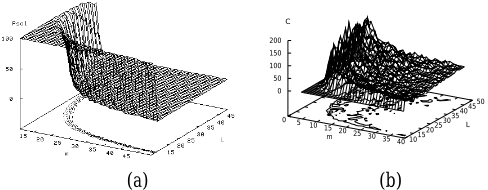
This search process shows a phase transition for critical values of the number ✜ of constants ☎ ✑ 's in the universe, and the number ✢ of literals in the hypothesis ✁ [Hogg et al., 1996; Prosser, 1996; Botta et al., 1999]. The graph in the ✂ ✢ ✟ ✜ ✏ plane of the probability that a model of ✁ exists in a0 is reported in Figure 1(a), for a set of covering problems generated according to a random model described in [Botta et al., 1999]. In the following, we will refer to "phase transition" as to the locus of the points ✂ ✢ ✣ ✟ ✜ ✣ ✏ for which the probability that a model exists is ✦ ✧ ✩ ✪ ✬ ✮ ✡ ✰ . The phase transition is located in correspondence of the "waterfall" in Figure 1(a). To the left of the phase transition (in the YESregion, i.e., the high plateau in Figure 1(a)) almost any example verifies any hypothesis. To the right of the phase transition (in the low plateau, i.e., the NO-region) almost no example ✳ verifies any hypothesis. The steep step corresponds to the "mushy" region, where the probability of a model existing drops from 0.99 to 0.01.In this region, the complexity of the search reaches its maximum, as reported in Figure 1(b).More details can be found in [Giordana et al., 2000; Botta et al., 1999].

1 Verifying ✱ on ✲ is a Constraint Satisfaction Problem, which exhibits a typical phase transition [Williams and Hogg, 1994; Smith and Dyer, 1996; Prosser, 1996].

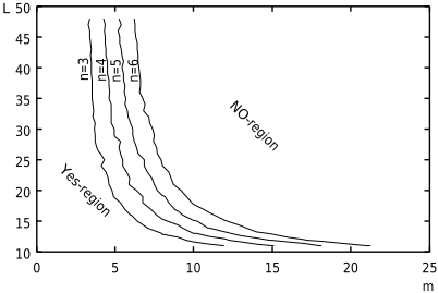
If the number of variables in the formulas changes, the location of the phase transition moves, as described in Figure 2.

3 Top-Down Induction

Let us consider a learning set ✴ and a conjunctive concept ✵ . Every pair ✂ a0 ✟ ✵ ✏ , with a0 ✷ ✴ , represents a covering test ✂ ✢ ✸ ✟ ✜ ✺ ✏ in the ✂ ✢ ✟ ✜ ✏ plane. A learning problem corresponds then to a cloud of points [Giordana et al., 2000]. In the special case that the number of constants in all examples is the same, the entire learning problem ✂ ✢ ✸ ✟ ✜ ✻ ✏ corresponds to a single point. In a similar way, any inductive hypothesis ✁ , built up by a learner in the attempt of finding ✵ , or at least a good approximation ✼ ✵ of it, can be represented as a cloud of points (or a single point) in the ✂ ✢ ✟ ✜ ✏ plane. Then, an induction process that proceeds by generating a sequence of hypotheses will describe a family of lines (or a single line) parallel to the ✢ axis.

In order to investigate how the presence of a phase transition in the ✂ ✢ ✟ ✜ ✏ plane may affect the behavior of a relational learner, an extensive experimentation has been done using a large set of artificially generated learning problems 2 . The results have been reported and discussed in [Giordana et al., 2000]. Here experimental setting and the findings are recalled, in order to state the base line for the work described in this paper.

The artificial learning problem set has been generated according to the following procedure. Given ✽ and ✾ , let ✂ ✢ ✟ ✜ ✏ be a point in the plane ✂ ✢ ✟ ✜ ✏ . A set of 451 points has been sampled in the plane ✂ ✢ ✟ ✜ ✏ . Then, for each point, a learning problem ✿ ❀ ❂ ❄ has been built up from the 4-tuple ✂ ✽ ✬ ❆ ✟ ✾ ✬ ❉ ✮ ✮ ✟ ✢ ✟ ✜ ✏ . A target concept ✵ with ✢ literals and ✽ variables has been built up, and then a training set ✴ ❄ and a test set ✴ ■ have been generated. Let ❏ be a set of ✜ constants; every example is a collection of ✢ relational tables of size ✾ obtained by sampling the binary table ❏ ❑ ❏ . In order to generate balanced training and test sets in each point of the ✂ ✢ ✟ ✜ ✏ plane, the random generation of the examples has been modified in order to obtain examples with models also in the NO-region, and examples without models also in the YES region (see [Giordana et al., 2000] for more details). The result has been the generation of training and test sets, ✴ ❄ and ✴ ■ , each one with 100 positive and 100 negative examples in each ✂ ✢ ✟ ✜ ✏ point.

The experimentation has been done primarily using FOIL [Quinlan, 1990]. A problem has been considered solved when the concept description found on ✴ ❄ was at least 80% accurate on ✴ ■ . However, other learners, such as SMART+ [Botta and Giordana, 1993] and G-NET [Anglano et al., 1998], have also been tried for comparison, reporting a strong agreement with FOIL both for the positive and for the negative cases. The results can be summarized as in the following. First, all tried learning strategies always end up generating concept descriptions lying on, or very close to, the edge of the phase transition. As discussed by [Giordana and Saitta, 2000], this phenomenon systematically occurs both in artificial and in real learning problems, as soon as the generated hypotheses involve more than three variables.

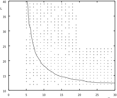
Second, a large "blind spot" located across the mushy region has been found: when the target concept lies there, no tried learner has been able to find any good generalization of the target concept (see Figure 3). Quite surprisingly, learning problems become again solvable by top-down induction when they are located in the NO-region, to the far right of the phase transition.

Finally, the computational complexity of matching inductive hypotheses lying in the mushy region may render the whole induction process infeasible. A possible way out has been proposed by [Giordana and Saitta, 2000], who suggested to use a stochastic algorithm for on-line estimation of the complexity, at the possible expenses of correctness.

2 All the artificial learning problems defined in this experimental setting are available at: http://www.mfn.unipmn.it/˜attilio/PROJECTS/phase- trans.html.

m

Figure 3: Relational learning with FOIL: Failure region (legend ".") and success region (legend "+"), for ✽ ✬ ❆ and ✾ ✬ ❉ ✮ ✮ . The contour plot corresponds to the value ✦ ✧ ✩ ✪ ✬ ✮ ✡ ✰ of the probability that randomly generated covering test is positive.

4 Why Top-Down Induction is Misled

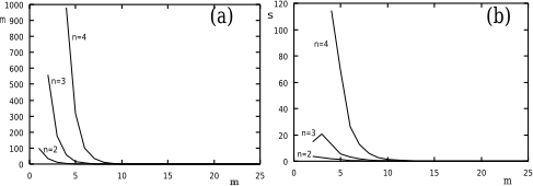
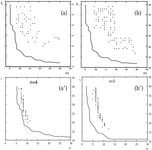
Before possibly designing new heuristics, it is necessary to clearly understand why FOIL and the other learners fail in the blind spot. A preliminary analysis showed that heuristics relying on the number of models, hypotheses have on the examples [Quinlan, 1990; Botta and Giordana, 1993; Rissanen, 1978], are not reliable in the YES-region, because both wrong and correct generalizations of the target concept have there similar numbers of models both on the positive and on the negative examples. In support to this claim, Figure 4(a) plots the average number ❙ of models a random hypothesis has as a function of ✢ , for ✜ ✬ ❉ ❱ . It is clear that an increase by 1 in the number ✽ of variables induces a large increase of ❙ and an even larger one on ❙ 's standard deviation ❲ . Actually, when ✽ ✬ ❆ the standard deviation is larger than the number of positive examples in the learning set. Then, even if we assume that generalizations of the target concept ✵ have at least one model more on the positive examples that on the negative ones, these generalizations cannot be distinguished from a purely random hypothesis. On the contrary, for hypotheses with 2 or 3 variables only, ❙ is much smaller, and we may expect that, provided that a correct generalization ✼ ✵ of ✵ with only two or three variables exists, it should be far easier to find it than any other one having four variables. This conjecture agrees with the fact that many solutions actually generated by FOIL have only three variables, even though the target concept is described by a formula with four variables.

A more detailed analysis is reported in Figure 5, where the line corresponds to the phase transition for ✽ ✬ ❆ . In Figure 5(a) the "+" denote the locations of a set of target concepts ✵ , whose description contains four variables. Figure ✰ ✂ ☎ ❩ ✏ shows the location of the solutions found by FOIL. Most of these solutions are generalizations of ✵ with four variables, because no acceptable generalizations with three or less variables could be found. On the contrary, Figure ✰ ✂ ❵ ✏ shows the locations of a set of target concepts whose description still contains four variables, but for which FOIL was able to find generalizations with no more than three variables (reported in Figure ✰ ✂ ❵ ❩ ✏ ). Problems in Figure 5(b) are then easier to solve than problems in Figure 5(a): this result corresponds to the fact that problems in Figure 5(a) are closer to the phase transition than problems in Figure 5(b). We observe that the probability of a problem being correctly approximated by a formula with only three variables increases with the number of literals in ✵ . In fact, when ✵ contains more literals, the number of its subformulas that are correct generalizations of ✵ increases as well; then, we may expect that at least some of them contains a number of variables smaller than ✵ 's. Moreover, the difficulty of a learning problem increases when ✜ decreases, whereas the critical value ✢ ✣ increases. When ✜ ❝ ❫ ✮ the only solutions found have three variables. In conclusion, most learning problems in the NO-region have been solved only because approximations with only three variables existed. When more than three variables are required, ✢ ✣ becomes larger, and available heuristics for top-down search are unable to grow valid inductive hypotheses starting from the YES-region. On the other hand, we could not find any bottom-up learning algorithm capable to cope with the complexity of working directly inside the NO-region.

5 A Stochastic Approach

In the absence of reliable heuristics, stochastic search may be a valid alternative, especially if combined with deterministic search. An example of an effective combination of a Monte Carlo search with deterministic search in the n-Queens problem can be found in [Brassard and Bratley, 1988]. The algorithm we propose is based on a two-step strategy. The first step creates a hypothesis ✁ ❢ with a complexity (number of literals) ❣ sufficient to reach the border between the YESregion and the mushy region; ✁ ❢ is the result of random sampling of the hypothesis space. The second step consists of a general to specific search, starting from ✁ ❢ according to a hill-climbing strategy guided by the information gain heuristics.

✐ ❥ ❦ ♠ ♥ ♦ ♣ a114 ✢ a115 ✉ ♦ ✽ ✇ Let ✼ ✵ ✣ ② ✍ ✬ ③ while halt condition does not hold do

1. Randomly generate a hypothesis ✁ ❢ close to the mushy region
2. Make ✁ ❢ more specific by following a hillclimbing strategy guided by the information gain. Let ✼ ✵ ④ be the locally best hypothesis found in trial ♣ .
3. if ✼ ✵ ④ is better than ✼ ✵ ✣ ② ✍ then replace ✼ ✵ ✣ ② ✍ with ✼ ✵ ④ .

end

If the target concept ✵ has a conjunctive description in the hypothesis space ⑤ , the Monte Carlo algorithm a115 ✉ ♦ ✽ ✇ is very likely, in the long run, to find ✵ , or at least a good generalization ✼ ✵ of it, correct on the learning set ✴ . Now, we want to answer the following question: assuming that the complexity ✢ ✸ and the number of variables ✽ ✸ in ✵ are known, what is the complexity we would expect from Algorithm a115 ✉ ♦ ✽ ✇ ? As "complexity" of the algorithm we mean the minimum number ⑧ ⑨ of trials necessary to reach a probability (1 - ⑩ ) of finding ✼ ✵ (or ✵ , as a specially lucky case). If we choose ❣ ✬ ✢ ✣ ❷ ❉ , there is a strong experimental evidence that a hill-climbing search, guided by the information gain, almost surely will find ✼ ✵ . This happens because the search explores the region where the information gain becomes reliable.

Let ✦ ❹ be the probability that ✁ ❢ is a sub-formula of ✵ , then the probability ✦ ❺ ✸ ❻ ④ ❼ of finding ✼ ✵ in nomore than ♣ steps is given by the expression:

Given ✢ ✸ and ✽ ✸ , the probability ✦ ❹ can be estimated, for a generic number ❿ of literals, as the ratio ✦ ❹ ✬ ✾ ➀ ✂ ✢ ✸ ✟ ✽ ✸ ✟ ❿ ✟ ➂ ✏ ➃ ✾ ➅ ✂ ✢ ✸ ✟ ❿ ✟ ➂ ✏ , where ✾ ➀ ✂ ✢ ✸ ✟ ✽ ✸ ✟ ❿ ✟ ➂ ✏ is the number of sub-formulas of ✵ with ❿ literals and ➂ variables (❫ ➆ ➂ ➆ ✽ ), and ✾ ➅ ✂ ✢ ✸ ✟ ❿ ✟ ➂ ✏ is the total number of formulas in the hypothesis space with ❿ literals and ➂ variables. An analytical expression for ✾ ➀ ✂ ✢ ✸ ✟ ✽ ✸ ✟ ❿ ✟ ➂ ✏ and ✾ ➅ ✂ ✢ ✸ ✟ ❿ ✟ ➂ ✏ has been given in [Serra, 2000], under the assumption that all predicates are binary. Using such expres-

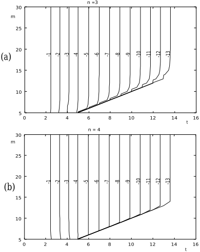
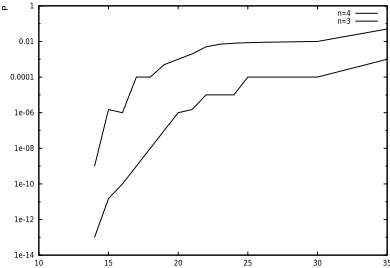
sions, the contour plot of Figure 6 have been obtained for the ratio ➋ ✂ ✢ ✸ ✟ ✽ ✸ ✟ ❿ ✟ ➂ ✏ ✬ ✾ ➀ ✂ ✢ ✸ ✟ ✽ ✸ ✟ ❿ ✟ ➂ ✏ ➃ ✾ ➅ ✂ ✢ ✸ ✟ ❿ ✟ ➂ ✏ setting ✽ ✸ ✬ ❆ , ➂ ✬ ❴ and ➂ ✬ ❆ . It is immediate to verify that ➋ ✂ ✢ ✸ ✟ ✽ ✸ ✟ ❿ ✟ ➂ ✏ decreases exponentially with ❿ , while it remains constant with respect to ✢ , after an initial exponential decay for small values of ✢ . The value ✦ ❹ can be obtained from Figure 6 by setting ❿ ✬ ❣ . As ❣ ✬ ✢ ✣ ❷ ❉ depends upon ✜ (see Figure 1), ✦ ❹ depends upon ✜ ✣ , too. The plots of Figure 7 report the dependency of ✦ ❹ upon ✜ ✣ for in the case of ➂ ✬ ❴ (dotted line), and in the case of ➂ ✬ ❆ (continuous line). For ✽ ✬ ❴ the phase transition occurs for smaller values of ✢ ✣ than for ✽ ✬ ❆ . Consequently, the values of ✦ ❹ for ➂ ✬ ❴ are order of magnitude larger than for ➂ ✬ ❆ . This explain why learning a concept with three variables only is much easier than learning a concept with four variables, as it has been stated in the previous section. We notice that the value ✜ ✣ is known when the learning examples are given, because ✜ ✣ is the average number of constants occurring in them.

6 Improving the Stochastic Search Algorithm

Expression (1) and the graphs in Figure 7 allow one to estimate the number ⑧ ⑨ of trials required to reach a confidence (1-⑩ ) that Algorithm a115 ✉ ♦ ✽ ✇ has found an approximation ✼ ✵ , provided that such an approximation exists. Then, the search can be planned as follows:

1. Assume an initial value ✽ ✸ for the number of variables in ✵ .
2. Estimate the number ⑧ ⑨ of trials necessary to reach the confidence level ✂ ❉ ❷ ⑩ ✏ . If ⑧ ⑨ is too high, stop, otherwise go to the next step.
3. Run a115 ✉ ♦ ✽ ✇ for ⑧ ⑨ trials.
4. If the result returned by a115 ✉ ♦ ✽ ✇ is acceptable, stop, otherwise increase ✽ ✸ by 1 and go to step 2.

We notice that the cost for generating and evaluating a hypothesis in the initial random sampling phase is much lower than the cost for the subsequent hill-climbing search. More specifically, the number of hypotheses to be generated and evaluated for the hill-climbing step can be estimated by:

being ➔ an integer that experimentally has been observed to range from ✮ to ❴ . In expression (2) the term ✂ ❉ ➓ ➔ ✏ is an estimate of the number of literals to be added to a hypothesis ✁ ❢ in order to cross the phase transition, whereas the term ✢ ✽ ✂ ✽ ❷ ❉ ✏ estimates the number of alternative specializations to be considered at each hill-climbing step.

Then, the number of hypotheses to be evaluated in the hillclimbing phase is from one to two orders of magnitude larger than the number of stochastic trials.

A second point worth noticing is that, assuming that the information gain heuristics is reliable for any hypothesis ✁ ❢ ↔ ↕ , it is also likely that ✁ ❢ itself be scored higher than the average when it is a sub-formula of ✵ .

m

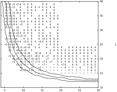
Figure 8: Results obtained by Algorithm ⑧ ➙ . The numbers denote the minimum value that was necessary to assume for ❣ in order to solve the learning problem. When the number is prefixed by "+", it means that ✽ ✬ ❆ has been assumed, otherwise ✽ ✬ ❴ . Symbol "." means that the problem has not been solved.

On the basis of the previous considerations we introduce a new algorithm, which can be more effective in practice than Algorithm a115 ✉ ♦ ✽ ✇ . Let ⑧ ⑨ be the number of trials estimated by (1) in order to reach a confidence ✂ ❉ ❷ ⑩ ✏ on the output of algorithm a115 ✉ ♦ ✽ ✇ . Let moreover ➜ ( ❉ ➆ ➜ ➆ ⑧ ⑨ ) be a user-defined parameter.

Algorithm ⑧ ➙

1. Create a set ➞ of ⑧ ⑨ hypotheseswith complexity ❣ .
2. Rank hypotheses in ➞ according to their information gain with respect to the formula ⑧ ♥ ➟ a0 .
3. Starting from the top ranked hypothesis, apply the hill-climbing specialization step to the ➜ best ranked hypotheses.
4. Return the best description ✼ ✵ .

Algorithm ⑧ ➙ tries to limit the number of hill-climbing steps to the hypotheses looking more promising, reducing thus the computational complexity. Of course, parameter ➜ is an arbitrary choice, and the confidence level ✂ ❉ ❷ ⑩ ✏ is guaranteed to be reached onlywhen ➜ ✬ ⑧ ⑨ . In practice, we have observed that using values of ➜ relatively small (➜ ✬ ❉ ➡ of ⑧ ⑨ ) ⑧ ➙ tends to produce the same results as for ⑧ ⑨ ✬ ➜ .

Algorithm ⑧ ➙ has been tested on the set of learning problems, reported in Figure 3, trying to solve the problems laying in the NO-region following the strategy described above. We started with the minimal hypothesis ✽ ✸ ✬ ❴ . Parameter ❣ has been set ❣ ✬ ❆ , which approximately corresponds to the edge of the phase transition for ✽ ✬ ❴ and ✜ ➥ ❴ ✮ . Even if for smaller values of ✜ our strategy foresees larger values of ❣ , it has been found that ⑧ ➙ was able to find a solution, with this setting, also for many problems where ❫ ✮ ➆ ✜ ➆ ❴ ✮ . Afterwards ➨ more expensive hypotheses has been progressively considered firstly increasing ❣ , until the value foreseen by the phase transition has been reached (or an excessive cost was foreseen) and then setting ✽ ✸ ✬ ❆ . A value ➜ ✬ ❉ ➡ of ⑧ ⑨ has been used everywhere. The results are reported in Figure 8. Comparing to Figure 3, we see that many problems lying in the blind spot have been solved. In practice almost all the problems above the phase transition and the line ✜ ✬ ❉ ❱ have been solved with a complexity larger as FOIL but still affordable. A cluster of 20 Pentium III (800 Mhz) has been used for the experiments, where every single problem required a time ranging from few minutes to several hours (an elapsed time comparable to FOIL on a sequential machine). When the problem was not solved we progressively increased the complexity of the hypothesis increasing ❣ .

7 Discussion

We have shown that combining stochastic search with local deterministic search it is possible to learn approximated concept descriptions where no known classical algorithm was successful. Even if the algorithm is used under the stringent assumption that a conjunctive concept description exists, it is not difficult to extend it in order to cope with more general concept descriptions. For instance, disjunctive descriptions can be learned by integrating ⑧ ➙ with a set covering algorithm as it is made in most relational learner [Quinlan, 1990; Botta and Giordana, 1993].

However, this is not the fundamental result that emerges from the framework we propose. In our opinion, the most important outcome is the method for estimating the complexity of a learning problem: given a specific hypothesis about the structure of the concept, we have a method for predicting the expected cost for testing the hypothesis. Moreover, a criterion for deciding on-line when stop testing the hypothesis is provided.

A second important result is a negative one, and concerns the possibility of learning descriptions with many variables. Even under the simplistic assumption that all predicates are relevant to the concept description, the task looks hard for many concepts requiring at least 4 variables. Increasing the number of variables, the complexity rises up exponentially. Considering the presence of irrelevant predicates, the analysis we performed still holds, but the the density of sub-formulas of the target concept close to the phase transition becomes even more tiny, and so the difficulty will increase further.