
Active Learning for Class Probability Estimation and Ranking
Proceedings of the Seventeenth International Joint Conference on Artificial Intelligence. Pages 911-919.
© 2001 International Joint Conferences on Artificial Intelligence
Abstract
For many supervised learning tasks it is very costly to produce training data with class labels. Active learning acquires data incrementally, at each stage using the model learned so far to help identify especially useful additional data for labeling. Existing empirical active learning approaches have focused on learning classifiers. However, many applications require estimations of the probability of class membership, or scores that can be used to rank new cases. We present a new active learning method for class probability estimation (CPE) and ranking. BOOTSTRAP-LV selects new data for labeling based on the variance in probability estimates, as determined by learning multiple models from bootstrap samples of the existing labeled data. We show empirically that the method reduces the number of data items that must be labeled, across a wide variety of data sets. We also compare BOOTSTRAP-LV with UNCERTAINTY SAM PLING, an existing active learning method designed to maximize classification accuracy. The results show that BOOTSTRAP-LV dominates for CPE. Surprisingly it also often is preferable for accelerating simple accuracy maximization.
- [Abe and Mamitsuka, 1998] Abe, N. and Mamitsuka, H. Query Learning Strategies using Boosting and Bagging. In Proceedings of the Fifteenth International Conference on Machine Learn- ing, pp. 1-9.
- [Angluin, 1988] Angluin, D. Queries and concept learning. Machine Learning, 2:319-342, 1988.
- [Bauer and Kohavi, 1998] Bauer, E., Kohavi, R. An Empirical Com- parison of Voting Classification Algorithms: Bagging, Boosting, and Variants. Machine Learning, 36, 105-142 (1998).
- [Blake et al., 1998] Blake, C.L. & Merz, C.J. UCI Repository of machine learning databases. Irvine, CA: University of California, Department of Information and Computer Science, 1998 [http://www.ics.uci.edu/~mlearn/MLRepository.html]. Link
- [Bradley, 1997] Bradley, A. P. The use of the area under the ROC curve in the evaluation of machine learning algorithms. Pattern Recognition, 30(7), 1145-1159, 1997.
- [Cestnik, 1990] Cestnik, B. Estimating probabilities: A crucial task in machine learning. In Proceedings of the Ninth European Con- ference on Artificial Intelligence, 147-149, Sweden, 1990.
- [Cohn et al., 1994] Cohn, D., Atlas, L. and Ladner, R. Improved generalization with active learning. Machine Learning, 15:201- 221, 1994.
- [Cohn et al., 1996] Cohn, D., Ghahramani, Z., and Jordan M. Active learning with statistical models. Journal of Artificial Intelli- gence Research, 4:129-145, 1996.
- [Cohen and Singer, 1999] Cohen, W. W. and Singer, Y. A simple, fast, and effective rule learner. In AAAI-99, 335-342, 1999.
- [Efron and Tibshirani, 1993] Efron, B. and Tibshirani, R. An intro- duction to the Bootstrap, Chapman and Hall, 1997.
- [Iyengar et al., 2000] Iyengar, V. S., Apte, C., and Zhang T. Active Learning using Adaptive Resampling. In Sixth ACM SIGKDD Intl. Conf. on Knowledge Discovery and Data Mining. 92-98.
- [Lewis and Gale, 1994] Lewis, D. and Gale, W. A. A sequential algorithm for training text classifiers. In ACM-SIGIR-94, 3-12.
- [Lewis and Catlett, 1994] Lewis, D. D., and Catlett, J. Heterogene- ous uncertainty sampling. In Proceedings of the Eleventh In- ternational Conference on Machine Learning, 148-156, 1994.
- [Provost et al., 1998] Provost, F.; Fawcett, T.; and Kohavi, R. The case against accuracy estimation for comparing classifiers. In Proc. of the Intl. Conf. on Machine Learning, 445-453, 1998.
- [Provost and Domingos, 2000] Provost, F. and Domingos P. Well- trained PETs: Improving Probability Estimation Trees. CeDER Working Paper #IS-00-04, Stern School of Business, NYU.
- [Quinlan, 1993] Quinlan, J. R.. C4.5: Programs for machine learn- ing.
- Morgan Kaufman, San Mateo, California, 1993.
- [Seung et al., 1992] H. S. Seung, M. Opper, and H. Smopolinsky. Query by committee. In Proceedings of the Fifth Annual ACM Workshop on Computational Learning Theory, 287-294, 1992.
- [Simon and Lea, 1974] Herbert A. Simon and Glenn Lea, Problem solving and rule induction: A unified view. In L.W. Gregg (ed.), Knowledge and cognitiom. Chap. 5. Potomac, MD: Erlbaum, 1974.
- [Turney, 2000] Turney, P.D. Types of cost in i nductive concept learning, Workshop on Cost-Sensitive Learning at ICML- 2000, Stanford University, California, 15-21.
- [Valiant, 1984] Valiant L. G. A theory of the learnable. Communica- tions of the ACM, 27:1134-1142, 1984.
- Winston, 1975].
- Winston, P. H. Learning structural descriptions from examples. In "The Psychology of Computer Vision", P. H. Winston (ed.), McGraw-Hill, New York, 1975.
- [Zadrozny and Elkan, 2001] Zadrozny B. and Elkan C. Learning and making decisions when costs and probabilities are both unknown. Technical Report No.CS2001-0664, Dept. of Computer Science and Engineering, UC San Diego, January 2001.
References were extracted automatically from the PDF and may contain errors.
Full text extracted automatically from the PDF; figures, tables and equations may differ. The PDF is the version of record.
1 Introduction
Supervised classifier learning requires data with class labels. In many applications, procuring class labels can be costly. For example, to learn diagnostic models experts may need to analyze many historical cases. To learn document classifiers experts may need read many documents and assign them labels. To learn customer response models, consumers may have to be given costly incentives to reveal their preferences.
Active learning processes training data incrementally, using the model learned "so far" to select particularly helpful additional training examples for labeling. When successful, active learning methods reduce the number of instances that must be labeled to achieve a particular level of accuracy. Most existing methods and particularly empirical approaches for active learning address classification problems-they assume the task is to assign cases to one of a fixed number of classes.
Many applications require more than simple classification. Decision-making often requires estimates of the probability of class membership. Class probability estimates (CPEs) can be combined with decision-making costs/benefits to minimize expected cost (maximize expected benefit). For example, in target marketing the estimated probability that a customer will respond to an offer is combined with the estimated profit (produced with a different model) [Zadrozny and Elkan, 2001]. Other applications require ranking of cases, to add flexibility to user processing. 1 We agree with Turney [Turney, 2000] that machine learning systems should be able to take into account various cost/benefit information, including decision-making costs as well as labeling costs.
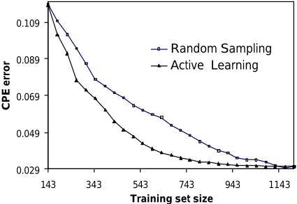
In this paper, we consider active learning to produce accurate CPEs and class-based rankings. Figure 1 shows the desired behavior of an active learner. The horizontal axis represents the number of training data, and the vertical axis represents the error rate of the probabilities produced by the model learned. Each learning curve shows how error rate decreases as more training data are used. The upper curve represents the decrease in error from randomly selecting training data; the lower curve represents active learning. The two curves form a "banana" shape: very early on, the curves are comparable because a model is not yet available for active learning. The active learning curve soon accelerates, because of the careful choice of training data. Given enough data, random selection catches up.
1 Classification accuracy has been criticized previously as a metric for machine learning research (Provost et al., 1998).
We introduce a new active learning technique, BOOTSTRAP-LV, which uses bootstrap samples of existing training data to examine the variance in the probability estimates for not-yet-labeled data. We show empirically across a wide range of data sets that BOOTSTRAP-LV decreases the number of labeled instances needed to achieve accurate probability estimates, or alternatively that it increases the accuracy of the probability estimates for a fixed number of training data. We also show that BOOTSTRAP-LV is surprisingly effective even for accuracy maximization.
2 Active Learning: Prior Work
The fundamental notion of active learning has a long history in machine learning. To our knowledge, the first to discuss it explicitly were [Simon and Lea, 1974] and [Winston, 1975]. Simon and Lea describe how machine learning is different from other types of problem solving, because learning involves the simultaneous search of two spaces: the hypothesis space and the instance space. The results of searching the hypothesis space can affect how the instance space will be searched. Winston discusses how the best examples to select next for learning are "near misses," instances that miss being class members for only a few reasons. Subsequently, theoretical results showed that the number of training data can be reduced substantially if they can be selected carefully [Angluin, 1988; Valiant, 1984]. The term active learning was coined later to describe induction where the algorithm controls the selection from a set of potential training examples [Cohn et al., 1994].
Input: an initial labeled set L, an unlabeled set UL, an inducer I, a stopping criterion, and an integer M specifying the number of actively selected examples in each phase. While stopping criterion not met /* perform next phase: */ Apply inducer I to L For each example { UL x x i i ∈ | } compute i ES , the effectiveness score Select a subset S of size M from UL based on i ES Remove S from UL, label examples in S, and add S to LOutput: estimator E induced with I from the final labeled set L
Figure 2: Generic Active Learning Algorithm
A generic algorithm for active learning is shown in Figure 2. A learner first is applied to an initial set L of labeled examples (usually selected at random or provided by an expert). Subsequently, sets of M examples are selected in phases from a set of unlabeled examples UL, until some predefined condition is met (e.g., the labeling budget is exhausted). In each phase, each candidate example UL x i ∈ is given an effectiveness score i ES based on its contribution to an objective function, reflecting the estimated magnitude of its contribution to subsequent learning (or simply whether it will or will not contribute). Examples then are ranked by their effectiveness scores and the top M examples are selected for labeling. Usually, multiple examples, rather than a single example, are selected at each phase due to computational constraints. Once examples are selected, their labels are obtained (e.g., by querying an expert) before being added to L, on which the learner is applied next.
Cohn et al. [Cohn et al., 1994] determine i ES based on identifying what they called the "region of uncertainty," defined such that concepts from the current version space are inconsistent with respect to examples in the region. The region of uncertainty is redetermined at each phase and subsequent examples are selected from this region. The main practical problem with this approach is that the estimation of the uncertainty region becomes increasingly difficult, as the concept becomes more complex. In addition, for complex concepts the region of uncertainty initially may span the entire domain before the concept is well understood, rendering the selection process ineffective . A closely related approach is Query By Committee (QBC)[Seung et al.,1992]: classifiers are sampled from the version space, and the examples on which they disagree are considered for labeling. However, QBC is a theoretical approach that poses computational and practical constraints. Particularly, it assumes the existence of hypotheses from the version space available for sampling, as well as noise-free data. Several other approaches also address learning for classification. These methods target examples for which predictions of class membership are evenly split (for binary classes) among an ensemble of classifiers, or alternatively examples for which a single probabilistic classifier assigns CPE near 0.5, as indicating class uncertainty. Specifically, Lewis and Gale [Lewis and Gale, 1994] proposed UNCERTAINTY SAMPLING where a probabilistic classifier is employed, and examples whose probabilities of class membership are closest to 0.5 are considered for labeling. Abe and Mamitsuka [Abe and Mamitsuka, 1998] generate a set of classifiers and then select examples for which the classifiers are close to being evenly split. An approach due to Iyengar et al. [Iyengar et al., 2000] directly estimates whether a classifier will assign an example to the wrong class. They employ a second classifier to assign classes to unlabeled examples, and examples are considered more informative for learning if estimated as being likely to be misclassified by the current ensemble of classifiers. These approaches are designed specifically for maximizing classification accuracy, not for optimizing CPEs or rankings, which are our concern.
The method most closely related to our technique was presented by Cohn et al. [Cohn et al., 1996] for statistical learning models. At each phase they compute the expectation of the variance of the model over the example space resulting from adding each candidate example to the training set. Our approach is similar in that it estimates variance, but instead of modeling the variance of the model over the input space, we estimate the "local" variance for each UL x i ∈ . The approach of Cohen et al. requires knowledge of the underlying domain, as well as the computation in closed form of the learner's variance, a constraint that renders it impracticable for arbitrary models. Our approach can be used for arbitrary models.
3 The Bootstrap-LV Algorithm
BOOTSTRAP-LV actively samples examples from UL to learn class probability estimates (CPEs). The description we provide here pertains to binary class problems where the set of class labels is { } 1 , 0 = C . As the discussion above indicates, we wish to add to L examples that are likely to improve the available evidence pertaining to poorly understood subspaces of the example space.
Ideally, the most direct indication of the quality of the current class probability estimate for example i x is the discrepancy between the estimated probability and its true probability. However, the true class probability for an instance is not known, nor is its actual class. Therefore we use the "local variance" (LV) to estimate this quality. Local variance refers to the variance in CPE for a particular example. If the estimated LV is high compared to that of other examples, we infer that this example is "difficult" for the learner to estimate given the available data, and is thus more desirable to be selected for learning. Otherwise, if the LV is low, we interpret it as an indication that either the class probability is well learned or, on the contrary, that it will be extremely difficult to improve. We therefore decrease the likelihood of these examples being added to L.
Given that a closed-form computation/estimation of this local variance may not (easily) be obtained, we estimate it empirically. We generate a set of k bootstrap subsamples [Efron and Tibshirani, 1993] j B , k j ,..., 1 = from L, and apply the inducer I to each subsample to generate k estimators j E , k j ,..., 1 = . For each example in UL we estimate the variance in CPEs given by the estimators { j E }. Each example in UL is assigned a weight, which determines its probability of being sampled, and which is proportional to the variance of the CPEs. More specifically, the distribution from which examples are sampled is given by ( ) [ ] { } R p p x p x D i k j i i j i s min , 1 2 / ) ( ) ( ∑= - = , where ) ( i j x p denotes the estimated probability an estimator j E assigns to the event
that example i x belongs to class 0 (the choice of performing the calculation for class 0 is arbitrary, since the variance for both classes is identical and hence the same result for ) ( i s x D is obtained for class 1); i p is the average k x p k j i j ∑ =1 ) ( ; min , i p is the average probability estimation assigned to the minority class by the various estimators, and R is a normalizing factor ( ) [ ] { } ∑ ∑ = = - = ) ( 1 min , 1 2 / ) ( UL size i i k j i i j p p x p R , so that s D is a distribution. This is the BOOTSTRAP-LV algorithm, shown in Figure 3.
Algorithm BOOTSTRAP-LV
- 1 Input: an initial labeled set L sampled at random, an unlabeled set UL, an inducer I , a stopping criterion, and a sample size M.
- B , k j ,..., 1 from L
- 2 for (s=1;until stopping criterion is met; s++) 3 Generate k bootstrap subsamples j =
- 4 Apply inducer I on each subsample j B and induce estimator j E
- 5 For all examples { UL x x i i ∈ | } compute
- 6 Sample from the probability distribution s D , a subset S of M exam-
ples from UL without replacement
- 7 Remove S from UL, label examples in S, and add them to L
- 8 end for
- 9 Output: estimator E induced with I from L
Figure 3: The BOOTSTRAP-LV Algorithm
There is one additional technical point of note. Consider the case where the classes are not represented equally in the training data. When high variance exists in regions of the domain for which the minority class is assigned high probability, it is likely that the region is relatively better understood than regions with the same variance but for which the majority class is assigned high probability. In the latter case, the class probability estimation may be exhibiting high variance due simply to lack of representation of the minority class in the training data, and would benefit from oversampling from the respected region. That is why we divide the estimated variance by the average value of the minority-class probability estimates min , i p . We determine the minority class once from the initial random sample.
4 Experimental Evaluation
We are interested primarily in comprehensible models, so for these experiments we use decision trees to produce class probability estimates. However, BOOTSTRAP-LV applies to any technique for learning CPEs. Particularly, the underlying probability estimator we use is a probability estimation tree (PET)-an unpruned C4.5 decision tree [Quinlan, 1993] for which the Laplace correction [Cestnik, 1990] is applied at the leaves. The Laplace correction has been shown to improve the CPEs produced by PETs [Bauer and Kohavi, 1998; Provost et al., 1998; Provost & Domingos, 2000].
When evaluating CPE accuracy, if the true underlying class probability distribution were known, an evaluation of an estimator's accuracy could be based on a measure of the actual error in probability estimation. Since the true probabilities of class membership are not known we compare the probabilities assigned by the model induced at each phase with those assigned by a "best" estimator, B E , as surrogates to the true probabilities. B E is induced from the entire set of examples (UL∪L), using bagged-PETs, which have been shown to produce superior probability estimates compared to individual PETs [Bauer and Kohavi, 1998; Provost et al., 1998; Provost & Domingos, 2000]. We compute the mean absolute error (MAE) for an estimator E with respect to B E 's estimation, denoted by BMAE. Spe-
estimated probability given by B E ; ) ( i E x p is the probability estimated by E, and N is the number of examples examined.
To evaluate its performance, we applied BOOTSTRAP-LV to 20 data sets, 17 from the UCI machine learning repository [Blake et al., 1998] and 3 used previously to evaluate rulelearning algorithms [Cohen and Singer, 1999]. Data sets with more than two classes were mapped into two-class problems. We compare the performance of BOOTSTRAP-LV against a method denoted by RANDOM, where estimators are induced with the same inducer and training set size, but for which examples are sampled at random. We show the comparison for different sizes of the labeled set L. In order not have very large sample sizes M for large data sets and very small ones for small data sets, we applied different numbers of phases for different data sets, varying between 10 and 30; at each phase the same number of examples was added to L. Results are averaged over 10 random partitions of the data sets into an initial labeled set, an unlabeled set, and a test set against which the two estimators are evaluated. For control the same partitions were used by both RANDOM and BOOTSTRAP-LV.
The banana curve in Figure 1 above shows the relative performance for the Car data set (where Active Learning refers to BOOTSTRAP-LV). As shown in Figure 1, the error of the estimator induced with BOOTSTRAP-LV decreases faster initially, exhibiting lower error for fewer examples. This demonstrates that examples actively added to the labeled set are more informative (on average), allowing the inducer to construct a better estimator with fewer examples. For some data sets BOOTSTRAP-LV exhibits even more dramatic results; Figure 4 shows results for the Pendigits data set.
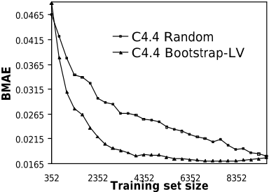
BOOTSTRAP-LV achieves its almost minimal level of error at 4500 examples. RANDOM requires more than 9300 examples to obtain this error level. For 5 of the 20 data sets, our approach did not succeed in accelerating learning much or at all, as is shown for the Weather data set in Figure 5. Note, however, that neither curve consistently resides above the other and the two methods' performance is comparable.
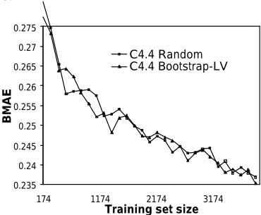
Table 1 presents a summary of our results for all the data sets. The primary motivation for applying active learning techniques is to allow learning with fewer examples. Table 1 provides a set of measures pertaining to the number of examples "gained" using BOOTSTRAP-LV instead of RANDOM. The second column shows the percent of phases in which BOOTSTRAP-LV produced the same level of CPE accuracy with fewer examples than RANDOM (we will call this "phases-gained"). The third and fourth columns show the percentage and number of examples gained by applying BOOTSTRAP-LV. The gain is calculated as the difference between the number of examples used by RANDOM and that used by BOOTSTRAP-LV to obtain the same CPE accuracy. The percentage is calculated based on the number of examples used by RANDOM. Because of the natural banana shape even for the ideal case, the performance of estimators induced from any two samples cannot be considerably different at the final phases, thus the averages as well as the phases-gained merely provide an indication of whether BOOTSTRAP-LV produces superior estimations. It is important also to observe the improvement at the "fat" part of the banana (where the benefit of active learning is concentrated). To allow a stable assessment we provide rather than the single best gain, the average of the largest 20% of the gains. Columns 5 and 6 of Table 1 show the average percent and average number (respectively) of examples gained for the top 20% gains. It is important that these figures be viewed in tandem with column 2 (phases-gained), to ensure that there is in fact a banana shape to the graph.
Table 1 also includes summary results pertaining to the error rates achieved by both methods for the same number of examples. Column 7 presents the average error reduction for the 20% of the sampling phases exhibiting the highest error reduction. For some data sets the generalization error for the initial training sets was small and was not considerably reduced even when the entire data was used for training (e.g., for connect-4, only 34% error reduction was obtained, from 11.7 to 7.7). We therefore also provide, in the last column, the top-20% error gain as a percentage of the reduction required to obtain the minimal error (the latter is referred to in the table as maximal gain). In the Adult data set, for instance, BOOTSTRAP-LV exhibited only 6.6% error gain (for the top 20%), but this improvement constitutes 25% of the possible improvement were the entire data set used for training.
| Examples | Error (%) | ||||||
|---|---|---|---|---|---|---|---|
| Data set | Phases with positive gain (%) | Avg % gained | Avg # gained | Top 20% % gained | Top 20% # gained | Avg top 20% (%) | Avg top 20% (% from maximal gain) |
| abalone | 92.5 | 34.9 | 574 | 76.9 | 1152 | 10.1 | 64.0 |
| adult | 96 | 17.8 | 302 | 30.2 | 585 | 6.6 | 25.0 |
| breast cancer-w | 100 | 23.8 | 44 | 51.6 | 110 | 9.3 | 41.0 |
| car | 89.6 | 23.3 | 155 | 35.4 | 281 | 31.3 | 53.3 |
| coding1 | 80 | 16.2 | 228 | 47.1 | 475 | 2.5 | 28.9 |
| connect-4 | 100 | 45.5 | 984 | 75.4 | 1939 | 9.5 | 27.5 |
| contraceptive | 93.7 | 18.4 | 55 | 42.3 | 129 | 5.7 | 31.3 |
| german* | 57.1 | 5.8 | 7 | 46.5 | 113 | 5.9 | 31.0 |
| hypothyroid | 100 | 64.6 | 705 | 69.0 | 1233 | 41.1 | 72.4 |
| kr-vs-kp | 100 | 18.1 | 37 | 27.1 | 57 | 25.5 | 30.8 |
| letter-a** | 72.4 | 14.5 | 229 | 24.8 | 529 | 10.4 | 26.0 |
| letter-vowel | 50 | 2.1 | 121 | 12.8 | 429 | 3.4 | 18.0 |
| move1 | 65 | 17.2 | 23 | 68.4 | 75 | 3.9 | 12.8 |
| ocr1 | 93.7 | 24.5 | 83 | 42.9 | 168 | 21.7 | 65.0 |
| optdigits | 94.4 | 24.5 | 412 | 50.0 | 762 | 32.6 | 47.8 |
| pendigits | 100 | 61.0 | 3773 | 68.6 | 5352 | 29.9 | 75.6 |
| sick-euthyroid | 93.1 | 45.2 | 600 | 70.2 | 924 | 26.2 | 58.5 |
| solar-flare | 64.2 | 13.5 | 25 | 41.5 | 58 | 6.3 | 9.9 |
| weather | 41.6 | -10.4 | -46 | 35.9 | 438 | 1.7 | 20.1 |
| yeast | 75 | 23.6 | 79 | 58.7 | 159 | 4.9 | 30.8 |
Table 1: Improvement in examples needed and improvement in error using BOOTSTRAP-LV
Since not all plots can be presented due to space constraints, we tried to express in the table various performance measures that would provide a comprehensive perspective. To assess BOOTSTRAP-LV's superiority we apply the combination of the following: phases-gained should be above 60%; both the average example and error gains should be positive, and the top-20% error reduction from the maximal gain should be 25% or higher. If phases-gained is between 40% and 60% we consider the methods to be comparable, and when it is below 40% we consider BOOTSTRAP-LV to be inferior. As can be seen in Table 1 (in bold), in 15 out of the 20 data sets BOOTSTRAP-LV exhibited superior performance. Particularly, in all but one phases-gained is 75% or above. In 13 of those, more than 30% of the examples were saved (for the top 20%), and in 9 data sets our method used less than 50% of the number of examples required for RANDOM to achieve the same level of accuracy. For the Sick-euthyroid data set, for instance, BOOTSTRAP-LV gradually improves until it requires fewer than 30% of the examples required by RANDOM to obtain the same level of accuracy. These results pertain to the top-20% improvement, so the maximal gain can be much higher.
For a single data set (Weather) BOOTSTRAP-LV exhibited a negative average examples gain. However, phases-gained, showing that BOOTSTRAP-LV uses fewer examples in 41% of phases examined, and Figure 5, both indicate that the two methods indeed exhibit comparable learning curves for this data set.
The measures pertaining to the number of examples gained and the error gain complement each other and may provide interesting insight. For instance, the number of examples gained can help evaluate the "difficulty" in error reduction in terms of the number of examples required by RANDOM to obtain such reduction. For example, although the average top-20% error gain for Connect-4 was less than 10%, Table 1 shows that it required RANDOM 984 additional examples on average to obtain the same improvement. A single data set, Letter-vowel, exhibited a negative average error gain. However, phases-gained is exactly 50%, indicating that RANDOM indeed does not exhibit superior performance overall. Both methods have similar learning curves.
We also assessed both methods with two alternatives to BMAE: the mean squared error measure proposed by Bauer and Kohavi [1998], as well as the area under the ROC curve [Bradley 1997] which specifically evaluates ranking accuracy. The results for these measures agree with those obtained with BMAE. For example, Bootstrap-LV generally leads to fatter ROC curves with fewer examples.
For those data sets in which BOOTSTRAP-LV exhibits insignificant or no improvement at all, training examples chosen at random seem to contribute to error reduction at an almost constant rate. Their learning curves have an atypical shape, as shown for the Weather data set in Figure 5, where additional examples bring an almost constant reduction in error rather than the expected decreasing marginal error reduction. This may indicate that it is easy to obtain good examples for learning, and any additional example contributes to error reduction equally, regardless of what or how many examples have been already used for training. Thus intelligent selection of learning examples is less likely to improve learning significantly.
5 Additional Experiments
Tree-based models offer a comprehensible structure that is important in many decision-making contexts. However, they often do not provide the best probability estimates. In order to assess BOOTSTRAP-LV 's performance on a better CPE learner, we experimented with bagged-PETs, which are not comprehensible models, but have been shown to produce markedly superior CPEs [Bauer and Kohavi, 1998; Provost et al., 1998; Provost & Domingos, 2000].
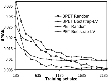
The results for the bagged-PETs model agree with those obtained for individual PETs. Particularly, for 15 of the data sets BOOTSTRAP-LV exhibited phases-gained of more than 65% (in 13 of those phases-gained is more than 75%). The average top-20% example gain was 25% or higher in 11 of those data sets. Only in two data sets is phases-gained less than 50%. Figure 6 shows a comparison between BOOTSTRAP-LV and RANDOM for individual PETs and for bagged-PETs. As expected, the overall error exhibited by the bagged-PETs is lower than for the PET, and for both models BOOTSTRAP-LV achieves its lowest error with considerably fewer examples than are required for RANDOM.
Described above, UNCERTAINTY SAMPLING [Lewis and Gale, 1994] was proposed for binary text classification. However, it too samples examples that are not well understood by the model. Since it was shown to improve a model's classification accuracy, it may improve the model's CPE as well. It therefore is interesting to compare the improvements exhibited by BOOTSTRAP-LV against UNCERTAINTY SAMPLING. We present a summary of the comparison results in Table 2, where all the measures are the same as in Table 1, except that the baseline comparison is UNCERTAINTY SAMPLING rather than RANDOM.
| Examples | Error (%) | ||||||
|---|---|---|---|---|---|---|---|
| Data set | Phases with positive gain (%) | Avg % gained | Avg # gained | Top 20% % gained | Top 20% # gained | Avg top 20% (%) | Avg top 20% (% from maximal gain) |
| abalone | 50.00 | 17.63 | 102 | 61.09 | 801 | 14.11 | 57.57 |
| adult | 69.23 | 9.56 | 69 | 35.03 | 284 | 11.13 | 27.18 |
| breast cancer-w | 55.56 | 10.90 | 15 | 49.37 | 144 | 20.20 | 43.91 |
| car | 62.50 | 9.95 | 6 | 50.46 | 68 | 36.30 | 43.26 |
| coding1 | 93.75 | 31.77 | 686 | 63.25 | 1027 | 6.74 | 49.26 |
| connect-4 | 89.47 | 43.89 | 1958 | 85.52 | 3230 | 54.02 | 82.91 |
| contraceptive | 50.00 | 11.76 | 21 | 54.87 | 126 | 10.01 | 29.13 |
| German | 81.25 | 24.74 | 69 | 48.14 | 146 | 8.12 | 37.63 |
| hypothyroid | 71.43 | 17.10 | 85 | 62.30 | 307 | 62.72 | 77.74 |
| kr-vs-kp | 94.74 | 33.90 | 90 | 57.71 | 144 | 60.43 | 64.07 |
| letter-a | 85.00 | 15.50 | 395 | 44.34 | 771 | 21.29 | 30.65 |
| letter-vowel | 100.00 | 63.80 | 11463 | 81.27 | 14210 | 44.97 | 43.41 |
| move1 | 100.00 | 39.96 | 194 | 62.89 | 247 | 16.29 | 36.26 |
| ocr1 | 100.00 | 35.86 | 146 | 51.90 | 256 | 34.30 | 61.75 |
| optdigits | 100.00 | 26.08 | 570 | 44.13 | 1359 | 34.91 | 58.16 |
| pendigits | 95.00 | 27.45 | 996 | 60.85 | 1636 | 38.30 | 58.03 |
| sick-euthyroid | 100.00 | 59.13 | 1093 | 84.12 | 1692 | 40.51 | 64.49 |
| solar-flare | 0.00 | -16.66 | -69 | -2.98 | -17 | -1.64 | -6.54 |
| weather | 56.25 | 6.32 | 3 | 35.06 | 351 | 1.98 | 24.74 |
| yeast | 53.33 | 7.74 | 3 | 40.38 | 121 | 6.03 | 28.88 |
BOOTSTRAP-LV exhibits markedly superior performance compared to UNCERTAINTY SAMPLING. Particularly, BOOTSTRAP-LV is superior in 14 of the data sets, and in 5 data sets the methods exhibit comparable performance, where phases-gained for BOOTSTRAP-LV between 50% and 60%.
UNCERTAINTY SAMPLING exhibits superior performance in one data set, Solar-Flare, for which it consistently produces better probability estimations.
In 9 out of the 14 data sets in which BOOTSTRAP-LV was superior, the average top error reduction was more than 30%. These results demonstrate that BOOTSTRAP-LV has a solid advantage when compared to UNCERTAINTY SAMPLING for class probability estimation. Moreover, for several data sets UNCERTAINTY SAMPLING'S performance was inferior to that of RANDOM. It is important to emphasize once again that indeed UNCERTAINTY SAMPLING was not designed to improve class probability estimation, but rather to improve classification accuracy.
We also compared the performance of UNCERTAINTY SAMPLING against BOOTSTRAP-LV for improving classification accuracy. Since BOOTSTRAP-LV was found to improve CPEs, a similar effect may be obtained for classification accuracy, but not necessarily: BOOTSTRAP-LV may select examples to improve class probability estimation even when the estimated decision boundary required for classification is already well understood, thereby "wasting" examples that do not improve classification accuracy.
Our results for classification accuracy show that in 11 data sets BOOTSTRAP-LV exhibited superior performance for accuracy maximization. UNCERTAINTY SAMPLING was superior in 7 data sets and the methods exhibited comparable performance for the remaining two. These results indicate that although BOOTSTRAP-LV is not uniformly superior to UNCERTAINTY SAMPLING for classification tasks, it should be considered a viable alternative-it often yields much better performance. Interestingly, in most cases where BOOTSTRAP-LV does not dominate, it performs better in the initial phases, whereas UNCERTAINTY SAMPLING surpasses BOOTSTRAP-LV in later phases. This phenomenon is demonstrated in Figure 7 for the Breast-Cancer data set.
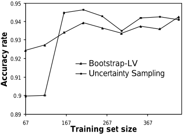
Recall that UNCERTAINTY SAMPLING uses the CPEs to determine the potential contribution of an example for learning. Therefore, its performance will be sensitive to CPE accuracy. Poor CPEs produced in the initial phases undermine the data selections by UNCERTAINTY SAMPLING. On the other hand, in later phases, more accurate probability estimations allow the selection process to focus in on the decision boundary. BOOTSTRAP-LV, on the contrary, focuses early on improving the CPEs, and therefore performs well even very early on the learning curve; however, later on it indeed "wastes" examples to improve CPE.
In light of this behavior, a better strategy for actively improving classification accuracy may be a hybrid approach: BOOTSTRAP-LV is applied in initial phases and UNCERTAINTY SAMPLING later. "When to switch?" is an open question.
6 Conclusions and Limitations
We introduced a new technique for active learning. BOOTSTRAP-LV was designed to use fewer labeled training data to produce better class probability estimates from fewer labeled data. We showed empirically that it does this remarkably well. We also showed that BOOTSTRAP-LV is competitive with UNCERTAINTY SAMPLING even for accuracy maximization. Inspecting these last results also suggests a hybrid strategy that may be even more effective than either technique alone.
BOOTSTRAP-LV was designed to identify particularly informative examples to use for training in order to economize on labeling costs to obtain higher CPE accuracy. It does not address computational concerns, as do Lewis and Catlett [Lewis and Catlett, 1994]. Indeed BOOTSTRAP-LV is a computationally intensive approach, because of the need to induce at each phase multiple models from a set of bootstrap samples. Yet, because of the typical shape of the learning curve, beyond a certain training set size the marginal error reduction is insignificant, whether active learning or random sampling is employed. Thus, intelligent selection of examples for learning is only critical in the early part of the curve, where a relatively small number of examples are used for training. Therefore, as long as the number of training examples remains relatively smallmultiple model inductions from these samples do not constitute a considerable computational toll. Moreover, BOOTSTRAP-LV provides an appropriate solution whenever labeling costs are more important than computational costs, for example, when the primary concern is to obtain accurate CPE or ranking with minimal costly labeling.
Acknowledgments
We thank Vijay Iyengar for helpful comments and IBM for a Faculty Partnership Award.
@inproceedings{ijcai2001p125,
  title     = {Active Learning for Class Probability Estimation and Ranking},
  author    = {Saar-Tsechansky, Maytal and Provost, Foster J.},
  booktitle = {Proceedings of the Seventeenth International Joint Conference on
               Artificial Intelligence, {IJCAI-01}},
  publisher = {International Joint Conferences on Artificial Intelligence},
  editor    = {Bernhard Nebel},
  pages     = {911--919},
  year      = {2001},
  url       = {https://ijcai.org/proceedings/2001/125},
}
TY - CPAPER TI - Active Learning for Class Probability Estimation and Ranking AU - Saar-Tsechansky, Maytal AU - Provost, Foster J. T2 - Proceedings of the Seventeenth International Joint Conference on Artificial Intelligence, IJCAI-01 PB - International Joint Conferences on Artificial Intelligence PY - 2001 SP - 911 EP - 919 UR - https://ijcai.org/proceedings/2001/125 ER -Copied
Machine-readable versions of this paper, for tools and AI agents:





