An Experimental Study of Phase Transitions in Matching

1 Introduction

Recent investigations have uncovered that several classes of computationally difficult problems, such as K­ Satisfiability problems (K-SAT) [Cheeseman et al., 1991; Crawford and Auton, 1996; Freeman, 1996; Selman and Kirkpatrick, 1996], Constraint Satisfaction Problems (CSP) [Smith and Dyer, 1996; Williams and Hogg 1994; Prosser, 1996], graph K-coloring problems [Cheeseman et at., 1991; Hogg, 1996], and the decision version of the Traveling Salesperson problems [Gent and Walsh, 1996; Zhang and Korf, 1996], show a phase transition with respect to some typical order parameter, i.e., they present abrupt changes in their probability of being solvable, coupled with a peak in computational complexity [Hogg et al., 1996].

Marco Botta

Dipartimento di Informatica Universita di Torino Corso Svizzera 185 10149 Torino, Italy

Lorenza Saitta

Dipartimento di Scienze e Tecnologie A vanzate Universita del Piemonte Orientale Corso Borsalino 54 15100 Alessandria, Italy

The identification of a phase transltton may have important consequences in practice. In fact, the standard computational complexity of a class of problems is a pessimistic evaluation, based on worst-case analysis. The investigation of phase transitions can provide information on single instances of the class, moving the focus from the maximum complexity to a typical complexity of instances. The location of the phase transition divides the problem space into three regions: one in which the probability of existence of a solution is almost zero, and then it is "easy" to prove unsolvability; another region, where many alternative solutions exist, and then it is "easy" to find one; finally, a third one, where the probability of solution changes abruptly from almost I to almost 0, potentially making very difficult to find a solution or to prove unsolvability.

Goal of the present work is to experimentally investigate the emergence of phase transition phenomena in the problem of matching a First Order Logic (FOL) formula to a universe, in order to possibly find one of its model. More specifically, we extend the work of Prosser [ 1996] on CSP along two directions. Firstly, we investigate in depth the relation between formula complexity and universe complexity, and secondly, we compare complexities in a deterministic and a stochastic search approach.

The basic motivation for studying the matching problem is that it is a basic step in learning structured concept descriptions from a set of positive and negative examples [Michalski, 1980]. The exponential (in time and/or space) complexity of this task severely limits the types of concepts that can be learned and used. Then, an effort to better understand the source of this complexity might suggest new and more effective learning strategies. Even though we keep in sight this ultimate goal, we limit ourselves, in this paper, to present results on the matching problem per se.

2 Problem Definition

A class of problems for which phase transittons have been investigated is that of Constraint Satisfaction Problems (CSP) [Williams and Hogg, 1994; Smith and Dyer, 1996; Prosser, 1996]. In a CSP, values are to be assigned to n variables { x 1 , x2 , .. . , Xn}, knowing that each variable xk can take values in an associated set Ak of cardinality Lk. A set R = { R., R2, .... , Rm} of constraints on variable values is given. The problem consists in finding a substitution for each variable such that all the constraints in R are satisfied. A relation R involving variables { x;, ... , xi} is represented as a table, in which the allowed tuples of values {a;, ... , ai} are specified. Any tuple not occurring in the table is not allowed. If all the relations are binary, the CSP is called binary [Williams and Hogg, 1994; Prosser, 1996; Smith and Dyer, 1996].

Two parameters are usually defined in order to account for the constrainedness degree of a CSP: constraint density and constraint tightness [Prosser, 1996]. When dealing with a binary CSP, the constraints can be represented as edges on a graph with n vertices, each one corresponding to a variable. The graph has n(n-1 )/2 possible edges; several constraints on the same pair of variables can be reduced to a unique one. By denoting by c the actual number of different edges activated on the constraint graph, the constraint density p1 [Prosser, 1996] is defined as:

Parameter p1 belongs to the interval [0, I], with 0 corresponding to no constraints, and I corresponding to the case in which all possible pairs of variables are constrained. For a constraint involving the pair of variables { x;, xi}, the tightness of the constraint is the fraction of value pairs ruled out by the constraint itself. If N is the cardinality of relation R(x;, xi), the constraint tightness p2 [Prosser, 1996] is defined by:

where L is the cardinality of the set of constants occurring in the universe.

It is immediate to see that the matching problem is a CSP. Finding a solution for a CSP can be formalized as a search on a variable assignment tree. Solution nodes can only exist at level n, both for the CSP and for the matching problem.

Formulas we consider are existentially quantified, conjunctive formulas, of the type 3x[ <p(x)], with n variables (from a set X) and m atomic predicates (from a set P). Given a universe U, consisting of a set of relations (tables) containing the extensions of the atomic predicates, formula <p(x) is satisfiable if there exists at least one model in U. In learning relations, a formula is an inductive hypothesis and a universe is a positive or negative example of the concept to learn. Then, in the learning problem, each hypothesis generated by the learner has to be matched against all the training examples, each one corresponding to a different universe. In Machine Learning, conjunctive formulas are the basic components of a global concept description, consisting of the disjunction of a number of them.

The following simplifying assumptions have been adopted in this framework:

• Each variable x., x2, .·. , Xn ranges over the same set A of constants, containing L elements (IAI = L).
• Only binary predicates are considered.
• Every relation in U has the same cardinality, namely it contains exactly N tuples (in this case, pairs of constants).

Instances of the matching problem (consisting of a formula <p and a universe U) have been generated according to the procedure described in the following. Given X and P, with the additional constraint m ~ n -1, the generation of a formula <p involves two steps. First, a skeleton <p, is deterministically constructed, using (n - I) predicates from the set P:

The skeleton guarantees that the resulting formula is not disjoint, i.e., that <p, cannot be partitioned into two subformulas with disjoint sets of variable names. Afterward, all the remaining (m-n+ I) predicates in P are added to <p, , randomly, uniformly, and without replacement (inside each predicate) selecting their arguments from the set X. With this procedure we obtain a formula:

where variables xi and xk belong to set X, and are such that j < k. The generated formulas contain exactly n variables and m conjuncts, and the same pair of variables may appear in more than one predicate.

Considering now a universe U, each relation in U is constructed by creating the Cartesian product A x A of all possible pairs of values, and selecting N pairs from it, uniformly and without replacement. In this way, a same pair cannot occur twice in the same relation.

In summary, the matching problems we consider are defined by a 4-tuple (n, m, L, N). From preliminary studies by the authors (see also [Prosser, 1996]), it emerged that the phase transition location depends upon a combination of p1 and p2: In the present experimentation, we have directly considered the parameters L (number of constants occurring in the universe) and m (number of predicates occurring in a formula), and we have explored points in the whole (L, m) plane, by keeping n ·(number of variables) and N (cardinality of the relations in the universe) constant.

3 Experimental Setting and Results

The exploration of the plane (L, m) has been done by considering a mesh covering the region corresponding to the Cartesian product of the sets L E [I 0,50] and m E [5 ,50]. For each of the 1886 points, 100 problems have been generated, according to the procedure described in Section 2, for N = 100 and n = 4, 6, 10, 12 and 14. The values for the number n of variables have been chosen consistent with those actually employed in learning relations in machine learning, where a value n = 10 is rarely depassed. Notice that the generation procedure requires that m ;:: n-1 and the non repetition of pairs in relations requires that L 2 ;:: N.

3.1 Probability of Solution

As the type of search algorithm does not affect the probability of a problem being solvable, but only the ease to find a solution (if any), we describe in Figure 1, the 3dimensional plot of the probability of solution P soh as a function of L and m, for n = 10. For each point in the mesh, P,01 has been evaluated as the fraction of solvable problems among all the generated ones.

Some contour level curves have also been reported in the (L,m) plane; the leftmost curve corresponds to P, 0 J = 0.85 and the rightmost one to P,01 = 0.15. The graphs in Figure I have several noteworthy characteristics, first of all, their striking steepness . The transition from Psol = 1 to P,01 = 0 occurs in the region bounded by the contour level curves.

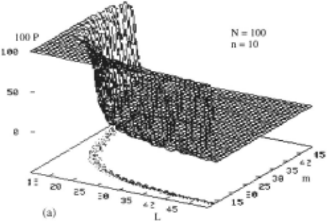
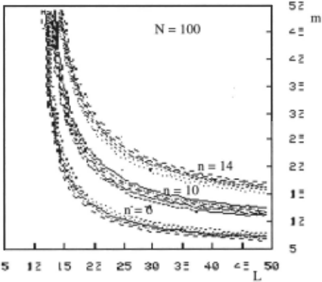
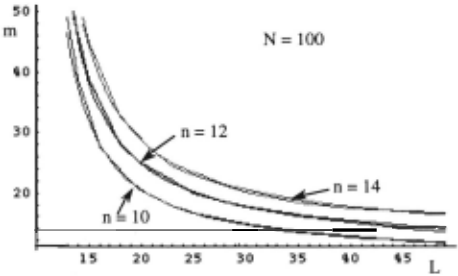
To the left of these curves, the problem has always a solution, whereas to the right of them no solution could ever be found . The second characteristic is the regularity on the horizontal planes: the projection on the (L, m) plane is a very smooth curve with a hyperbolic behavior. Finally, by increasing the number of variables, there is a shift toward up and right, causing an enlargement of the solvable problems region, as it can be clearly seen in Figure 2.

To perform the search, two algorithms have been used, a deterministic one, Ad , and a stochastic one, A, and run on every problem instance.

3.2 Deterministic Search

The deterministic algorithm Ad explores the search tree depth-first, and stops as soon as a solution is found, or it explores the whole tree up to level n, if no solution exists . Given a formula q>(x) with the structure (2), the search tree 't is built up in such a way that each level corresponds to the assignment of values to the variables, considered in the sequence (x1, ... , x.) 1 . The search proceeds through the construction of partially satisfied subformulas of <Pi(x), until either the whole q>(x) is satisfied or unsatisfiability is proved. We start with a subformula

where 132 is the subformula of q>.(x) that contains those predicates with arguments (x~ox2). Obviously, subformu~a 132 may be empty, if the pair (x1,x2) does not occur m q>.(x). If q>2(x~ox2) is satisfiable, we consider variable x3 and subformula

q>3(X~oX2,x3) = q>2(X~oX2) 1\ U2(X2,X3) 1\ I33(XJ,X2,X3) where 133 is the subformula of q>.(x) containing the predicates with arguments (x~ox2), (XJ,X3) or (x2,x3). The process goes on in the same way until variable Xn is considered.

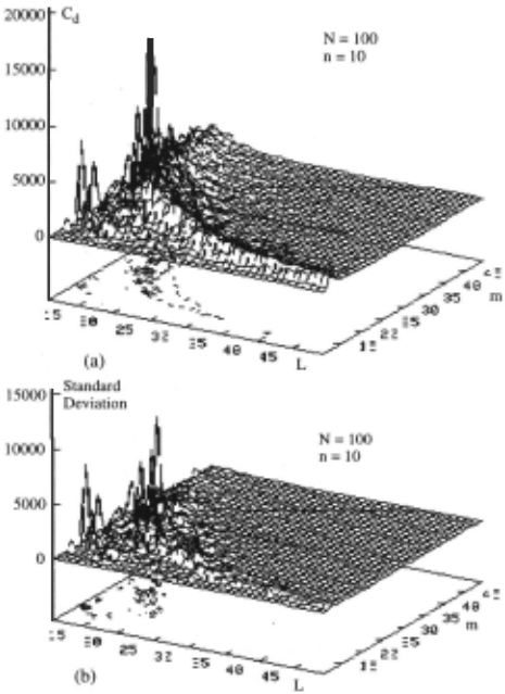
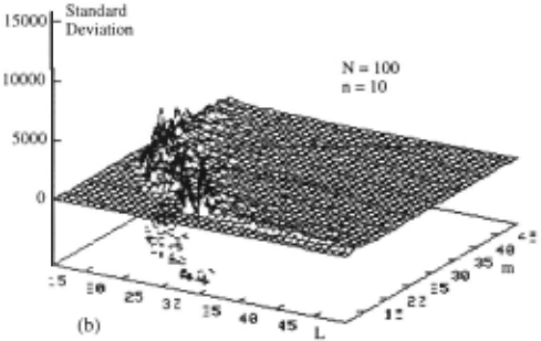
In Figure 3(a), the graph of the complexity Cd of the search, measured as the number of expanded nodes in the tree, and averaged over 100 repetitions, is reported. As we can see, the shape and location of the region of higher complexity roughly matches that of the transition in probability, but it is more irregular and much broader, like a "mountain chain". In particular, we may notice that in the bottom-left corner, where the easy problems should be, there are a few quite high peaks, even though there is a general decrease of the complexity. Similar phenomena have been observed before, for instance by Gent and Walsh [1994]. Finally, inside the "mountain", there is a large variability among different instances, witnessed by the variance plot, reported in Figure 3(b). As one may expect, the highest variance occurs in correspondence of the highest peaks.

1 Actually we have also experimented with different variable orderings, for example by considering the most constrained variables first. Even though reduction in complexity may results from applying such heuristics, the qualitative behaviour does not change. Hence, we have preferred to use a simpler search algorithm, because efficiency of the searcher in not on focus in this paper.

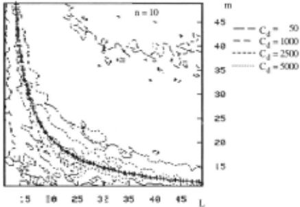
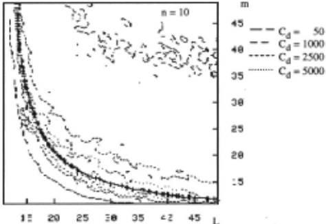
Finally, in Figure 4, the c.ontour level plots of the probability of solution and those of the complexity are superimposed, in order to localize the maximum complexity with respect to the curve at Psol = 0.5.

As we can see, the maximum complexity, apart from the anomalous peaks in the bottom-left corner, coincides with the line at Psol = 0.5, as it has been previously found [Hogg et al., 1996].

3.3 Stochastic Search

Given the large size of the search tree, and the possibility for a solution to be anywhere inside, one may wonder under what circumstances a stochastic search algorithm may be effective. The use of a stochastic algorithm is also suggested by the added value offered by the on-line estimation of interesting quantities related to the tree, for instance its size [Bailleux, 1998].

The specific search algorithm used here is a Monte Carlo algorithm MC, which explores one path on the search tree, starting from the root and ending in a leaf v, which may or may not be a solution. Since we remember the already explored leaves, this path sampling is performed without replacement. Algorithm MC is a Monte Carlo one [Brassard and Bratley, 1988], because it always provides an answer y, but the answer may be incorrect.

The same graphs as in Figures 3 and 4 are reported in Figures 5 and 6, for the complexity C, of the stochastic search.

From Figure 5(a) we can see that the complexity C, has a more regular behaviour than Cd. In fact, Cs's highest peaks are lower than Cd's (finding confirmed by the lower variance in Figure 5(b)), even though, on average over all instances, the complexities are almost the same for the two cases. For instance, one may notice that the complexity of the stochastic search is higher than that of the deterministic one in the region of low L values and high m values .

An interesting aspect of the greater regularity of the stochastic search is the total absence of anomalous peaks in the "easy" region, which is absolutely flat. This more regular behaviour clearly appears in Figure 6, the analogous of Figure 4. The contour level plots are much cleaner and the maximum complexity neatly coincides with the line at P,01 = 0.5.

15000 c,

10000

(a)

N = 100

n = 10

L

4 Discussion of the Results

The results described in the previous section extends the ones presented in [Prosser, 1996] . In fact, by using a higher granularity in the mesh and collecting a larger variety of measures, some new phenomena emerge. First of all , it is impressive the very large variance in the complexity which is almost of the size of the average complexity. This can be explained considering the structure of the formula, which is not captured by the order parameter p1· Depending on how the literals aggregate, the complexity can be extremely high or very low in correspondence of the mushy region. A similar behavior has been already mentioned in [Hogg et al. , 1996] . However, the phenomenon seems even more evident here because of the double variability due to both the universe structure and the formula structure. It is worth noting that the stochastic algorithm exhibits a much lower variance, while the mushy region is sharper and the contours are more regular. The explanation is that the variability due to the localization of the solutions in the search tree is averaged by the specific stochastic strategy, while the variability due to the formula structure is not affected by it.

IS

2:Q

25

~~~~~

3Z 3: m

4-5

Finally, from Figure 2 it clearly emerges a quasi­ hyperbolic relation between m and L. This pattern was partially visible in some diagrams reported in [Prosser, 1996], but in Figure 2 it is better defined, being the explored region wider and more finely sampled. In the following we give a theoretical interpretation of this phenomenon. Let us consider the region of the phase transition, i.e., the line in the (L,m) plane corresponding to P,01 = 0.5. This curve has a meaning only when m ~ (n-1) and L 2 ~ N. We can try to justify the shape of this curve as follows . When P,01 = 0.5, the average number of solutions is about I [Gent and Walsh, I996; Walsh, 1998], i.e., half of the instances are unsolvable, whereas the other half has a small number of solutions.

According to our procedure for generating problem instances, this situation corresponds to the case in which the first binary relation may be any, the following (n-2) ones have one element partially constrained by the preceding ones (constants must be chained, in order to have a solution), and the remaining (m-n+ I) have one element completely fixed, because they contain only variables already appeared in the first part of the formula. Then, the probability of this event is proportional to:

By taking the natural logarithms, we obtain from (3) a relation between m and L at the phase transition:

In (4) the constant parameter a has been estimated (for each n) from a unique point on the experimental curve, obtaining the degree of fit shown on Figure 7. It is interesting to note that, for a = I, this relation coincides with the one previously obtained by the authors, following a methodology similar to Prosser's [I996] .

5 Conclusions

In this paper, the complexity of matching First Order conjunctive formulas has been analyzed, obtaining a relation linking the parameters describing the syntactic complexity and the semantic complexity. More specifically, we have identified the presence of three regions: a region (a) where the complexity is low and usually formulas are satisfiable; a region (b) where the complexity is very high and the probability of solution quickly moves from I to 0; a region (c) where the complexity is low again but the probability of solution is zero, in practice.

In order to correctly interpret such results, it is worth noting that P,01 = 0 in region (c) only means that it is very rare to find a formula satisfiable in this region when the formulas and universes are extracted at random. On the contrary, it is always possible to construct a matching problem that has solution in region (c), and also it is always possible to construct problems in region (a), which do not have solutions.

Therefore, the existence of a group of solvable problems in region (c) or of unsolvable problems in region (a) has to be interpreted as the evidence of a regularity, which potentially can be learned by a relational learner. Vlasie [ 1996) has pointed out a similar phenomenon for graph 3-colorability. On the contrary, the presence of solvable and unsolvable problems in the mushy region is exactly what one expects from a random instance generation. Moreover, the high complexity in region (b) is a serious obstacle for any learning algorithm.

Finally, the high variability inside the phase transition suggests to use, when necessary, on-line estimation of the expected complexity, therefore complementing the information derivable from a static localization in the phase plane of the problem to be solved. This dynamic estimation would allow the search to be interrupted when the expected complexity is likely to exceed the available computational resources.