Semi-Quantitative Comparative Analysis

1 Introduction

In many situations it is important to compare the be­ havior of dynamical systems. A population biologist , for instance, may want to predict the consequences of the introduction of a new species into an ecosystem. For an engineer monitoring a chemical process, it may be critical to know whether a particular perturbation could explain observed deviations from the normal behavior.

If quantitative models and precise quantitative infor­ mation about the initial conditions are available, a com­ parative analysis (CA) of the behaviors of the systems is straightforward. One simply compares the behav­ iors predicted by means of numerical simulation at the time-points of interest. Often, however , the available information about the systems is incomplete. In such cases we can resort to qualitative models to describe the systems, predict behaviors from an initial qualita­ tive state by means of qualitative simulation [Kuipers, 1994], and use qualitative CA techniques to compare the behaviors [Weld, 1988; Neitzke and Neumann, 1994; de Jong and van Raalte, 1997].

A disadvantage of qualitative CA techniques is the imprecision of their conclusions, which hampers their upscalability. When comparing the behaviors of more complex systems, with several structural differences and differences in initial conditions, de Jong and van Raalte's CEC* is likely to generate a large number of possible comparative behaviors. Besides these ambiguities, due to the qualitative nature of the available information, it only characterizes differences as higher or lower, without giving an indication of their magnitude.

Hidde de J ong France

IN RIA Rhone-Alpes 655, avenue de l'Europe 38330 Mont bonnot Saint Martin

In this paper we introduce SQCA, a technique which arrives at more precise conclusions than ·qualitative CA techniques, while retaining their ability to deal with incomplete information. The technique exploits semi­ quantitative information about the systems, in the form of numerical bounds on the variables and functions oc­ curring in the models. Although SQCA will be presented as a self-contained technique, it can also be integrated as a filter on comparative behaviors into a qualitative CA algorithm. The implementation of SQCA has been used to answer CA questions involving structural differences in combination with differences in the initial conditions of the systems.

The presentation starts with a brief review of semi­ quantitative simulation, since semi-quantitative models and behaviors form the input of SQCA (sec. 2). Semi­ quantitative CA is basically a constraint propagation process. Sec. 3 describes how the requisite constraints are derivable from the models and behaviors of the sys­ tems to be compared. The SQCA algorithm is given in sec. 4, together with guarantees on its correctness and convergence. In sec. 5 the results obtained by means of SQCA are presented, followed by a discussion in sec. 6.

2 Semi-quantitative simulation

We employ the semi-quantitative simulation techniques Q2+Q3, which function as filters on qualitative be­ haviors obtained by means of QSIM [Kuipers, 1994; Berleant and Kuipers, 1997]. Although other simulation techniques could have been used as well (e.g. , [Vescovi et al. , 1995]) , we have chosen Q2+Q3 because they produce a semi-quantitative annotation of the behaviors while preserving their underlying qualitative structure.

The models used for semi-quantitative simulation are semi-quantitative differential equations (SQDEs) , that is, qualitative differential equations (QDEs) enhanced with numerical information (fig. 1) . We use a nota­ tion for QDEs which emphasizes their abstraction from ODEs and which simplifies the propositions in later sec­ tions. Besides the basic qualitative constraints in QSIM, it allows the use of composite qualitative constraints [Vatcheva and de Jong, 1999]. For instance, the con­ straint

Figure 1: QDEs for an object fired upwards in a gravitational field, where the gravitational field is (a) constant, (b) height-varying and completely specified, and (c) height-varying and incompletely specified. In (b) and (c) friction is taken into account , whereas in (a) it is neglected. (d) Ranges and envelopes which turn the QDEs into SQDEs. The variable h stands for height above the Earth surface, v for velocity, a for acceleration, g for gravitational constant, r for Earth radius, x for distance from the center of the Earth, and k for a constant dependent on the air density p, projected area A of the object in the direction of motion, object mass m , and drag coefficient c.

the latter two being composite constraints themselves. Generally speaking, we deal with constraints QV(y) = f( QV(x1 ), .. . , QV(xn)) (or QV(y) = f( QV(x))), where f is a qualitative constraint between the variables y,X!, . .. ,Xn.

The semi-quantitative information completing the QDE takes several forms. In the first place, numeri­ cal ranges are added to landmarks. For a landmark li, range(li) is defined as an interval [I;, li] with li, li E JR* . Second, envelopes can be added to monotonic function constraints in the QDE. An envelope(!) of a mono­ tonic function is defined as a pair of functions[_,/, with f(x):::; f(x):::; f(x), for all x in the domain of f.

- Q2 is a technique which uses the ranges and envelopes of the SQDE to refine a qualitative behavior tree pro­ duced by QSIM. Given ranges for the variables in the ini­ tial qualitative state, it builds a constraint network and propagates the initial ranges through this network. The constraint network relates the variables at each distin­ guished time-point through constraints on their ranges. Constraint propagation is achieved by recursively eval­ uating the constraint expressions by means of interval arithmetic and by updating the range of a landmark through intersection of the present range and the newly calculated range. Q2 either rules out qualitative be­ haviors or produces qualitative behaviors in which the qualitative values are annotated with numerical ranges, so-called semi-quantitative behaviors (SQBs) .

Q3 improves upon the results obtained by means of Q2 by following an approach called step-size refinement.

First, it locates or creates a gap in a semi-quantitative behavior, that is, it takes a pair of adjacent distinguished time-points ti and ti+l , such that ti < l i+I · Then, it interpolates a new state in this gap at an auxiliary time­ point taux , ti < taux < ti+l > and provides initial ranges for the qualitative value of the variables at taux· The newly created state adds new landmarks and constraints to the constraint network. A new round of constraint propagation by means of Q2 results in a refined or re­ futed semi-quantitative behavior.

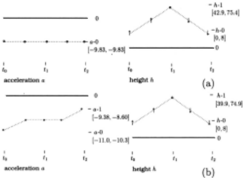
Fig. 2 shows two semi-quantitative behaviors produced by QSIM and Q2+Q3 from the models in fig. 1. Both behaviors describe an object falling back to its initial height, in the first case in a constant gravitational field without friction and in the second case in a height­ varying gravitational field with friction.

3 RIV s and RIV constraints

3.1 Relative interval values

Consider two SQBs, either topologically equal or topo­ logically different [Weld, 1988]. Topologically equal be­ haviors show the same sequence of transitions between qualitative states and the (shared) variables have the same qualitative value in the corresponding states of this sequence.

Let t0 , ... , tn and t0 , . . . , tm be the sequences of dis­ tinguished time-points in the first and the second SQB, respectively. The behaviors are compared at meaningful pairs of comparison [de Jong and van Raalte, 1997]. A pair of comparison pe is a pair (t, i) of time-points in the behavior of the first and second system. 1 It is meaning­ ful if one of the following conditions is satisfied: (1) t and tare the initial time-points to and to; (2) t and tare the end time-points tn and tm; or (3) t and tare time-points at which a variable reaches the same landmark 0, -oo or oo in both systems. Pairs of comparison can be ordered by a partial ordering relation: pea ::::5 pel, iff to :::; t 1 and to :::; t1, where pco = (to, to) and pel = (tl,il)· pel is called a successor of pco. A comparison of the behav­ iors in fig. 2 yields the meaningful pairs of comparison pea = (to, to), pel = (tb t1), and pe2 = (t2, t2), with PCo ::::5 pel ::::5 pe2.

A comparison of the shared variables of the systems at a pair of comparison gives rise to relative interval val­ ues (RIVs). They provide an estimate of the difference ~x(pe) = x(i) - x(t) of variables x at pe = (t, i) .

Def. 1 The RIV of a shared variable x at a pair of com­ parison pe is defined as range(~x(pe)).

The RIV s at a pair of comparison are related to each other, and to the RIV s at predecessor and successor pairs of comparison. The RIV constraints expressing these relations are derived from the SQBs and the SQDEs of the systems which we want to compare. Several types of RIV constraints exist.

3.2 Constraints from SQBs

A direct way to obtain a range for the difference of a vari­ able at a pair of comparison is to examine the numerical information in the states of the SQBs.

Prop. 1 At pe = (t , i) the RIV of xis given by

A special case of this proposition is the difference in the duration of the behavior fragments T and T, defined by two successive pairs of comparison pco = (t0 , t0 ) and pel= (t1,t1 ):

1 As a notational convention, ~ denotes variables in the behavior of the second system.

The behaviors in fig. 2 show .that the range of the acceleration in the first and second system is range(a(t0 )) [-9.83, -9.83] and range(a(to)) [-11.0, -10.3], respectively. Applying prop. 1 at peo yields range(~a(pco)) = [-1.17, -0.47] .

3.3 Constraints from SQDEs at a pair of comparison

Suppose the qualitative value of a shared variable x is constrained in the first and second system as follows:

where f and g represent qualitative constraints, and r and s are vectors of variables. We will allow the models of the two systems to be structurally different, so f and g as well as r and s may be different .

In order to derive an RIV constraint from (2), f and g need to be made comparable first. This is attained by bringing f and g in the form of a single constraint, the so-called comparison constraint. Let q be the vec­ tor of variables occurring both in r and s, and a a vec­ tor of newly introduced auxiliary variables with specified qualitative values, so-called comparison values. The con­ straints f and g are comparable through a comparison constraint h,

under the following condition: h is satisfied iff f and g are satisfied for every QV(r), QV(s) given the compar­ ison values QV(a), QV(a) .

In contrast with [de Jong and van Raalte, 1997], the existence of such a comparison constraint can be guar­ anteed. The set of basic qualitative constraints is re­ stricted and for every pair of f and g a comparison con­ straint can be easily found due to the simple form of f and g. When f and g are composite, a comparison con­ straint is obtained by decomposing f and g into basic constraints and composing the corresponding compari­ son constraints into a composite comparison constraint h [Vatcheva and de Jong, 1999].

The acceleration constraint from the model in fig. 1(b) can be decomposed as in (1) and the acceleration con­ straint in fig. 1(a) as

The comparison constraint of the first qualitative constraints in (1) and (4) is defined as QV(p1) = -QV(g)QV(a1) with comparison values QV(a1) = (1 , std) and QV(a1) = QV(f 2 ji 2 ). The compari­ son constraint of the second constraints is Q V (a) = QV(p1) + QV(a2) with comparison values QV(a2) = (0, std) and QV(a2) = QV(p2). Their composition de­ fines has

Prop. 2 Suppose that QV(x) and QV(i ) are con­ strained by f and g , as in (2). Let h be the comparison constraint off and g. The RIV of x at pc = (t , i) is given by:

with dq and d4 vectors of partial derivatives of the func­ tion corresponding to the comparison constraint, i.e. , dq ,i = 8~, h(mq, rna) and da,j = -/.;;h(mq, ma) . 2 Further, mq, lies between Qi ( t) and tli ( i) , and ma, between aj (t) and aj(i) .

Proof. The constraints in (3) are abstractions of the mathematical equations

where h is a continuously differentiable function. Sub­ tracting x(t) and x(i) and applying the generalized mean value theorem, one finds

where mqi lies between Qi(t) and tJi(i), and maj between aj (t) and aj(i) . 0

Ranges for the partial derivatives of h are derived from interval extensions Dq,i and Da,j of dq,i and da,j, respec­ tively [Moore, 1979]. It can be easily shown that such interval extensions always exist and are uniquely speci­ fied [Vatcheva and de Jong, 1999].

In this way,

Similar expressions are obtained for range( maj) and range(da,j)·

In the example above we find at peo the RIV constraint

' ' 2 2 A with span(al(to) , al(to)) span(1 , r jx (to)) , range(~al(PCo)) range(f 2 jx 2 (io)) - [1, 1], and range( ~a2 (peo)) = range(p2 ( io)) .

2 Throughout this paper h is used to refer both to con­ straint and the mathematical function from which the con­ straint is abstracted. Whenever a confusion is possible, we explicitly speak of the constraint h or the function h.

3.4 Constraints from SQDEs between pairs of comparison

Between pairs of comparison the behavior of a shared state variable x is determined by the derivative con­ straints in the SQDEs:

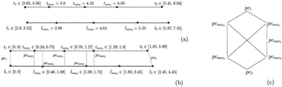
Derivative constraints give rise to additional RIV con­ straints. Consider the pairs of comparison peo = (to, to) and pc1 = (t1, t1) , which define primitive behavior frag­ ments [to, t1] and [to, i 1], that is, behavior fragments without intermediary distinguished time-points. The in­ tervals will usually contain auxiliary time-points taux, E ]to, tt[ and iaux1 E]to, i1 [, which have been interpolated during simulation (sec. 2) .

Since in general to f= io , we will synchronize the be­ havior fragments first by means of a procedure which shifts the uncertainty in t0 and t0 to subsequent time­ points. The ranges of the synchronized time-points t 8 in the behavior fragment of the first system are defined as: range(tg) = [0, OJ, range(ti) = [h -to, t1 - tJ], and range(t~ux.) = [taux, - to, taux, - tJ] . Synchronization of the behavior fragment of the second system is accom­ plished in the same way. We will henceforth assume that the behavior fragments have been synchronized already.

We now introduce auxiliary pairs of comparison by means of the auxiliary time-points. These pairs of com­ parison allow one to improve the prediction of differences at qualitatively important time-points.

Def. 2 Suppose two systems are compared over primi­ tive behavior fragments defined by PCo and pc1 with n and m auxiliary time-points. Setting tauxn+J = t1 and iauxm+J = tt, we define auxiliary pairs of comparison

where 1 ~ i ~ n+1, 1 ~-j ~ m+1, and 1 ~ k ~ n+m+l.

Notice that we introdqce auxiliary pairs of comparison only conditionally. The condition taux, ~ i1 for PCauxk ensures that taux, is a time-point really occurring in the (synchronized) behavior fragment of the second system.

Fig. 3(a) shows primitive behavior fragments of an ob­ ject launched upwards. Q3 has interpolated three aux­ iliary time-points in each behavior fragment . The syn­ chronized behavior fragments and the auxiliary pairs of comparison are shown in fig. 3(b). The pairs of compar­ ison have been ordered with respect to the ~-relation .

With the help of the auxiliary pairs of comparison, the RIV of the shared state variable x at pc1 can be expressed in terms of the RIV s of x at auxiliary pairs of comparison between peo and pc1.

Prop. 3 Given the qualitative constraints (6) and k auxiliary pairs of comparison defined by def. 2. The RIV

of the shared state variable x at pcaux, (1 ~ i ~ k) and pc1 is defined as follows

where peaux, are direct predecessor pairs of comparison of PCaux; and pel, and PCauxo is set to PCo·

Proof. Let PCaux; = (taux;, taux;), PCauxi (tauxi, tauxi ), peauxi ~ PCaux;. Applying the mean value theorem for x and x in the time interval [tauxi, taux;] and subtracting the resulting expressions we get

where mtaux, mt aux E] taux., tauxJ Taking into account that r and s are qualitatively uniform between the ad­ jacent time-points to, t 1 and io, i 1 , respectively, and hence between the auxiliary time-points taux,, taux;, we conclude that r( mt aux) E span( r( tauxJ, r( taux.)) and s(mtaux) E span(s(tauxJ, s(tauxJ) . The expression above can then be transformed into

Since pcaux; may have more than one direct predeces­ sor pcauxi, there can be a number of estimations of the RIV of x at PCaux, computed by means of the RIV of each PCauxi . Hence, the RIV of X at PCaux; is given by the intersection of these estimations.

The proof of the second part of the statement is accomplished in an analogous way. 0

In the example of fig. 3 the proposition contributes 6 RIV constraints for each of the variables h and v.

As a special case, consider the situation that x is con­ stant in both systems, i.e.

Without proof we add the following proposition.

Prop. 4 Suppose that QV(x) and QV(i) are con­ stants, as in (7), and we compare the systems over behav­ ior fragments determined by peo and pc1 . The RIV of x at pe1 is now simply range(6.x(pel)) = range(6.x(peo)) .

For example, for the gravitational constant g we have range(6.g(peo)) = range(6.g(pel)) = [0, OJ.

3.5 Redundancy of constraints

Prop. 2 relies on the mean value theorem to obtain more precise estimates of the RIV s of variables at pairs of com­ parison. O~e can prove that there are situations in which the RIV constraints thus defined do not improve upon the RIV constraints defined by prop. 1. In particular, this occurs when the SQDEs are completely specified. An SQDE is completely specified when it does not con­ tain monotonic function constraints.

Theor. 1 Suppose the SQBs of two completely spec­ ified systems are compared. If range(6.x(pc))t is the RIV of a variable x at pc determined by prop. 1, and range(6.x(pc))H2 the same RIV determined by prop. 1 and 2, then range(6.x(pc)h ~ range(6.x(pc)h+2·

Since the models are completely specified, h does not contain monotonic function constraints. In this case the corresponding function and its partial derivatives are real-valued rational functions with corresponding natu­ ral interval extensions. The statement is then proved by analogy of the proof of prop. 2 using basic propositions from interval arithmetic.

4 SQCA algorithm

The algorithm for semi-quantitative comparative analy­ sis takes as input two behaviors SQB ,SQB and the cor­ responding models SQDE,SQDE of the systems, where SQDE,SQDE are assumed to consist of basic qualitative constraints only. SQCA generates RIV s for all shared variables at the pairs of comparison from a set of ini­ tial RIV s. The algorithm consists of the following three steps:

1. Establish the meaningful pairs of comparison im­ plied by SQB and SQB.
2. Generate the RIV constraints from SQB, SQB and SQDE, SQDE, and build a constraint network.
3. Resolve the constraint network for the initial RIVs.

Prop. 1 to 4 define constraint schemata which are in­ stantiated in the second step to yield appropriate RIV constraints from SQB, SQB and SQDE, SQDE. 3 The constraints thus generated form a constraint network linking together the differences ~x of shared variables at the pairs of comparison.

In the third step the constraint network is resolved for the initial RIVs by means of the propagation algorithm included in Q2 (sec. 2) . The result of the constraint propagation is an RIV for each shared variable x at each pair of comparison pc. If some RIV is 0, the initial RIVs are not consistent with the models SQDE, SQDE and behaviors SQB, SQB from which the RIV constraints have been derived.

SQCA has been shown to be sound and incomplete [Vatcheva and de Jong, 1999]. Call range(~x(pc))out the range for shared variable x at pair of comparison pc that has been produced by SQCA. We now find:

Theor. 2 SQCA is sound, in that for any pair of solu­ tions of ODEs consistent with the SQCA input it holds that ~x(pc) E range(~x(pc)) out for all x and pc.

Theor. 3 SQCA is incomplete, in that for some value riv in range(~x(pc))out there may be no solutions of ODEs consistent with the SQCA input, such that ~x(pc) = riv.

Soundness is a consequence of the sound derivation of RIV constraints from SQDEs and SQBs {sec. 3) and the soundness of the constraint propagation algorithm. In­ completeness is caused by the possibility of excess width in interval arithmetic [Moore, 1979) and the use of the weak mean value theorem in prop. 2 and 3.

An important property of SQCA is its convergence.

Theor. 4 The RIVs calculated by SQCA converge to a point value as the ranges in the initial qualitative states converge to a point value and the maximum step-size in the semi-quantitative behaviors converges to 0.

3 In order to obtain tighter bounds for the RIVs, prop. 2 is not only applied to qualitative constraints of type (2), but also to algebr~ically equivalent constraints.

The proposition rests on the convergence of Q3 and holds under the same conditions [Berleant and Kuipers, 1997].

5 Results

The SQCA algorithm has been implemented in Common Lisp. The program interacts with available implementa­ tions of QSIM and Q2, and our own implementation of Q3: it takes semi-quantitative behaviors produced by QSIM and Q2+Q3 as input and calls Q2 functions for building and resolving constraint networks. In contrast with the implementation of CEC* the process of deriv­ ing propagation constraints from the SQBs and SQDEs has been completely automated. This is possible due to the fact that the models in the SQCA input consist of basic constraints only.

In the first half of the table below the results of ap­ plying SQCA to the behaviors in fig. 2 are shown. The trajectory of an object fired upward in a constant gravi­ tational field without friction is compared with that in a height-varying gravitational field with friction (fig. 1{a­ b)). Although the initial height and velocity are incom­ pletely known in both systems (with ranges [0, 8] and [30, 35), respectively), they are known to be equal, so that the initial RIVs range(~h(peo)) and range(~v(peo)) are both [0, 0]. The SQCA results show that one can­ not predict with certainty whether the maximum height reached by the second object will be higher or lower, i.e. range(~h{pc1 )) = [-27.4, 27.8). The structural dif­ ferences work in different directions, the height-varying gravitational field tending to increase and friction tend­ ing to decrease range(~h{pc1 )) , while the uncertainty in the initial conditions is too large to distinguish between the two. The prediction of the difference in maximum height is more precise than that obtained in qualitative CA, however.

In the second half of the table two identical systems are compared, both described by the incompletely spec­ ified SQDEs in fig. 1{c). In this case the initial RIVs are range(~h{peo)) = [-4, -2] and range(~v{peo)) = [16, 20], which work in different directions. Can we tell whether the higher initial velocity compensates the lower initial height , even though our knowledge of the systems is incomplete? The results show that the maximum height is greater by [44.6, 136.8} in the second system (range(~h{pc1 ))) , so that the higher velocity compen­ sates the lower height. In this case, CEC* generates 15 comparative behaviors and does not unambiguously answer the question. After combining the comparative behaviors with the SQCA output, only 3 remain.

Omitting the RIV constraints from prop. 2 does not influence the results in the first example. How­ ever, for the incompletely specified models in the sec­ ond example SQCA gets worse results without these constraints: range(D.a(pc2)) = [-1.55, 3.87] instead of range(D.a(pc2)) = [-1.55, 3.56] . In both examples we ob­ tain worse results when the RIV constraints from prop. 3 are omitted. This shows that semi-quantitative CA can­ not be reduced to the trivial approach of subtracting simulation values at pairs of comparison (prop. 1).

SQCA has been tested on a number of examples, in­ cluding brittle fracture systems in fracture mechanics and prey-predator systems in population ecology. It successfully answers CA questions involving structural differences in combination with differences in the initial conditions of the systems.

6 Discussion and related work

SQCA borrows ideas from both semi-quantitative sim­ ulation and qualitative comparative analysis. As in Q2+Q3, the problem is reduced to a constraint prop­ agation problem. However, SQCA employs constraints dealing with ranges of value differences instead of ranges of values. The constraints are derived from a pair of models instead of a single model, with the additional complication that SQDE, SQDE may be structurally different and fragments of SQB, SQB unsynchronized.

To our knowledge, only de Mori and Prager [1989) have studied the semi-quantitative comparative analysis of dynamical systems, but their approach is restricted only to linear, time-invariant systems and employs semi­ quantitative information on a coarser level of granularity. Moreover, unlike SQCA their technique for qualitative perturbation analysis cannot deal with structural differ­ ences between systems and with topologically different behaviors.

Given that the SQCA input is valid, the RIVs range(D.q(pc))out produced by SQCA contain the ac­ tual difference D.q at pc (soundness) . However, they may overestimate this value due to a loss of informa­ tion in the process of generating and propagating con­ straints (incompleteness). By using techniques for the solution of interval CSPs that are more powerful than the constraint propagation algorithm currently employed in SQCA (e.g., [Benhamou and Older, 1997)), the problem of excess width could be reduced. Also, the RIV con­ straints defined by prop. 3 can be improved by replacing in some cases the mean value theorem with explicit in­ tegration [Vescovi et al., 1995].

Even when the predicted RIV s are as tight as possi­ ble given the input, they may turn out not to be precise enough. The convergence theorem shows that by inter­ polating additional auxiliary time-points in the SQBs, and thus introducing new auxiliary pairs of comparison and new RIV constraints, we can improve the results of SQCA. This suggests an approach in which the preci­ sion of SQCA's predictions is dynamically increased by iterating between semi-quantitative simulation and comparative analysis.

7 Conclusions and further work

SQCA is a technique for the semi-quantitative analysis of dynamical systems which is both able to deal with in­ completely specified models and arrive at precise predic­ tions by exploiting available numerical information. The technique has a solid mathematical foundation which fa­ cilitates proofs of correctness and convergence proper­ ties. SQCA has been fully implemented, including the derivation of propagation constraints.

Future work will concentrate on the improvement of the precision of the technique, along the lines mentioned in the previous section, and its integration into a system for the model-based analysis of scientific measurements (see [de Jong et al., 1998)).