
Perturbation Analysis with Qualitative Models
Proceedings of the Eleventh International Joint Conference on Artificial Intelligence. Knowledge Representation. Pages 1180-1185.
© 1989 International Joint Conferences on Artificial Intelligence
Abstract
Perturbation analysis deals with the relationships between small changes in a system's inputs or model and changes in its outputs. Reverse simulation is of particular interest, determining how to achieve desired outputs by perturbing inputs or model parameters. Some applications of this type of analysis are suggested. Perturbation analysis is developed in the context of continuous systems whose dynamics, over small ranges of the system's behaviour, can be represented by linear models. All variables and signals are represented by intervals with qualitative end points. Qualitative linear models are introduced to represent time-varying systems. These representations permit the use of network consistency algorithms to solve perturbation analysis problems. This paper is dedicated to the memory of Dr. Murdoch McKinnon, late of CAE Electronics Ltd. and Concordia University, who faithfully supported this research since its beginning.
- Table 4: QILs for selected signals and cut-points References
- Alef-83]
- Alefeld, G. ; Herzberger, J. Introduction to Interval Computations; Academic Press, 1983 [Bobr-84
- Bobrow, D. G. (Editor) Qualitative Rea- soning about Physical Systems. A Bradford Book, The MIT Press, 1985. Reprinted from Artificial Intelligence Journal; Vol. 24; 1984.
- Davis, E. Constraint Propagation with Interval Labels; Artificial Intelligence Journal; Vol. 32; pp. 281-332; 1987.
- de Kleer, J. ; Brown, J. S. A Qualitative Physics Based on Confluences; appears in [Bobr-85]; pp. 7, 83; 1985.
- Eykhoff, P. System Identification; J. Wiley & Sons; 1974
- Falk-88] Falkenhainer, B The Utility of Difference- Based Reasoning; Proceedings: AAAI, 1988
- Forbus, K. D. Qualitative Process Theory; appears in [Bobr-84]; pp. 85, 168; 1984.
- Forbus, K. D. Interpreting Observations of Physical Systems; IEEE Trans. on Systems, Man, and Cybernetics; Vol. SMC-17; pp. 350- 359; 1987.
- Friedland, B. Control System Design: An Introduction to State-Space Methods; McGraw- Hill Book Company, 1985
- Han, C.-C. ; Lee, C.-H. Comments on Mohr and Henderson's Path Consistenct Algo- rithm; Artificial Intelligence Journal; Vol. 36; pp. 125-130; 1988.
- Iwasaki, Y. ; Bhandari, I Formal Basis for Commonsense Abstraction of Dynamic Sysytems; Proceedings: AAAI, 1988
- Kuipers, B. J. Commonsense Reasoning about Causality: Deriving Behavior from Struc- ture; appears in [Bobr-84); pp. 169, 204; 1984.
- Kuipers, B. J. Qualitative Simulation; Artificial Intelligence Journal; Vol. 29; pp. 289- 338; 1986.
- Kuipers, B. ; Berleant, D. Using Incom- plete Quantitative Knowledge in Qualitative Rea- soning; Proceedings: AAAI, 1988
- Mack-77)
- Mackworth, A. K. Consistency in Net- works of Relations; Artificial Intelligence Jour- nal; Vol. 8; pp. 99-118; 1977.
- Mohr, R . ; Henderson, T. C. Arc and Path Consistency Revisited; Artificial Intelli- gence Journal; Vol. 28; pp. 225-233; 1988.
- Murthy, S. S. Qualitative Reasoning at Multiple Resolutions; Proceedings: AAAI, 1988 [Pavl-73)
- Pavlidis, T. Waveform Segmentation Through Functional Approximation IEEE Trans. on Computers; Vol. c-22; pp. 689-697; 1973
- Prager, R ; Belanger, P. ; De Mori, R. A Knowledge-Based System for Troubleshooting Real-Time Models; appears in Artificial Intelli- gence, Simulation and Modeling;
- Widman, L. E. ; Loparo, K. A. ; Nielsen, N. R. (editors); J. Wiley and Sons; 1989. [Raim-86) Raiman, 0. Order of Magnitude Reason- ing; Proceedings: AAAI, 1986
- Simm-86)
- Simmons, R. "Commonsense" Arithmetic Reasoning; Proceedings: AAAI, 1986 [Walt-75)
- Waltz, D. Understanding Line Drawings of Scenes with Shadows; appears in The Psychology of Computer Vision;
- Winston, P.H. (Editor) [Weld-88)
- Weld, D.S. Comparative Analysis; Artifi- cial Intelligence Journal; Vol. 36; pp. 333-374; 1988.
- Williams, B. C. MINIMA: A Symbolic Approach to Qualitative Algebraic Reasoning; Proceeding AAAI; 1988
References were extracted automatically from the PDF and may contain errors.
Full text extracted automatically from the PDF; figures, tables and equations may differ. The PDF is the version of record.
1. Introduction: Qualitative Perturbation Analysis
1.1 Reasoning about continuous systems
Most work on qualitative physics [Bobr-84] has been device-centered (e.g. electric circuits, tanks and pipes) with models derived from component topol ogy [deKl-84]. Inferences about the behaviour of a device are made by constraint propagation. Qualita tive reasoning about processes [Forb-84], models the behaviour of a system as the combined effect of active processes which describe the relations and influences between objects. However, a system is still considered as a collection of objects and rela tions between them. In QSIM [Kuip-86], continuous functions (over time) represent state variables and constraints model system structure.
Components and interconnections are not the only models for dynamic systems. In some continuous systems, state variables depend on the aggregate behaviour of many elements. For example, the aerodynamic forces on an aircraft are the result of integrating the forces caused by airflow · over the entire airframe. System models may be finite element approximations or differential equations; both types are useful for numerical simulations. Such models may be used in problem-solving, but are surely not the basis of human reasoning. When people design, control or diagnose such dynamic sys tems they use their understanding of physical princi ples and problem-solving skills. In particular, peo ple seem to reason about orders of magnitude of variables, and relations between variables and their rates of change. This paper considers how to make a computer program do the same.
1.2 Outline of the paper
This paper describes QP A and the representations and algorithms which it requires. References to related research are included throughout the paper. The remainder of this section introduces the notion of a perturbation to a system, discusses the types of models to which QPA is applicable, and summarizes the contributions of this research. Section two describes the qualitative representation of variables and signals, and the qualitative calculus. An exam ple QLM is introduced in section two. Perturbations of QLMs and a transformation to a CSPs are dis cussed in section three. Section four concludes with a summary and ideas for future work.
1.3 Perturbations and applications
Engineers are frequently interested in how a system responds to perturbations. Consider a system A whose behaviour during a manoeuvre is described by a set M of initial conditions, inputs and outputs. Note that inputs and outputs are signals. One type of anaJysis is to change an input or initial condition of a manoeuvre, or a parameter of the model, and perform a simulation to see the effects. A more dif ficult problem is to do the inverse. Given a desired perturbation on the outputs of a manoeuvre, how can this be achieved by perturbing inputs, initial conditions or model parameters? The representa tions and algorithms used in answering these types of questions are called Qualitative Perturbation Analysis (QPA) and are the subject of this paper.
QP A can be used to find causes of discrepancies between systems and models. If output discrepan cies can be expressed as perturbations, any input, initial condition or parameter modified by QP A can be considered a cause of the original discrepancies. There are many potential applications of QPA:
Design: A design model is being used to design a system A with desired behaviour M. If simulations do not match M, QPA can determine design changes so that A will meet its specification.
Diagnosis: Let A be a real, malfunctioning system, let M contain symptoms. If QP A discovers causes for the symptoms, any perturbed parameters are possible faults in A.
Validation: When A is a real system and M contains real measurements, QPA can be applied to perturb simulation parameters to improve their accuracy.
This research is part of a project studying AI techniques for validation of aerodynamic models (see (Prag-89] for an overview) .. A knowled~e-ba~ed assistant system, called the Fhte System, 1s bemg built for simulation engineers. QPA is designed for the key role of reasoning about discrepancies in simulations.
1.4 Linear models of a system
Models for qualitative reasoning about continuous systems should have several properties:
- (a) related to human mental models
- (b) represent a wide variety of systems
- (c) represent relations between variables
- (d) represent time-varying signals
- (e) amenable to aggregation by subsystem
- (f) can be instantiated given recorded signals
An appropriate class of models is fir~t order linear differential equations (FOLDEs), wh1ch have many applications in modern control theory. [~rie-.85] (e.g. to model spring-coupled masses, d1shllat10n columns etc.). For example, equations to model small motions in an aircraft's longitudinal axes are given in Figure 1. For some M a single set of FOLDEs may not be accurate, in which case M can be segmented and modeled by a sequence of FOLDEs, one per segment (see (Pr~g-89]). QPA is applicable to systems whose behavwur, af.ter seg mentation, can be modeled by FOLDEs w1th con stant coefficients.
Qualitative models can be derived from analytic models by representing all terms by qualita!ive values and interpreting equations as constramts (deKl-84], (Will-88]. Qualitative f:inear ~od.els (QLMs) are versions of FOLDEs, w1th a quahtahve representation for signals and gains (coefficients. of the FOLDEs are called gains). QLMs clearly satls~ properties (h), (c) and (d) above. Property (e) 1s discussed in [Iwas-88]. Given the model stru~ture and signals, gains can be estimated by. syste.m iden tification techniques [Eykh-74], thus (f) 1s sahsfied.
where
u : velocity along the x-axis,
(} : angle between the x-axis and the ground,
q : derivative of (},
a : angle of airflow over the wings,
o. : elevator control input,
Fthrust : engine thrust.
Figure 1: Aircraft longitudinal dynamics
Whether QLM's satisfy (a) is more difficult to argue. It does seem to be useful to reason about decoupled sub-systems, relative influences between variables, and relative magnitudes of signals. QLMs support these types of reasoning.
The relation between linear models and complex simulation models is discussed in [Prag-89]. A map ping from QLMs to complex models will in general be possible by exploiting the structure of the domain. Since this is a domain dependent problem, QP A is concerned only with linear models in their general form.
1.5 The QPA strategy
Given A and M, the first step of QPA is to compute a QLM L and the qualitative representation of sig nals in M. Knowledge of A is only used to deter mine the equations of L. Next, QPA uses L and a differentiation formula (see 2.4) to compute con straints on the derivatives of the QLM. Derivative constraints are critical to QPA since they constrain values of signals at successive time points. Third, output perturbations are applied (usually all at the same time point), making L inconsist~nt. '~:'he fi?al step of QPA is to formulate a constramt sahsfachon problem (CSP) and solve to find new values of sig nals, and possibly gains, consistent with _the p~rtur bations. The transformation to a CSP 1s des1gned such that the general algorithms of (Mack-77] (see also [Mohr-86] and [Han-88]) can be applied.
1.6 Contributions
This work makes contributions in three areas. First, QP A addresses the problem of inverse qualitative simulation, inferring input or model chan~es fr~m output perturbations, which is not covered m [Kmp86]. Comparative analysis [Weld-88] is also con cerned with forward simulation, taking a system behaviour and a perturbation to the model to predict output perturbations. QPA differs from difference based reasoning (Falk-88] since QPA is concerned with systems modeled by differential equations, not examples described by sets of axioms.
The second contribution is the use of QLMs to represent relations between qualitative variables. QLMs model system behaviour over time with a sin gle set of relations, rather than by a sequence of states (e.g. as in [Forb-87]). FOLDEs have many applications; their qualitative analogues may also be widely useful. Making useful inferences about per turbations requires a representation of real numbers with a finer granularity than the commonly used { -1, 0, +1}. QILs, with a qualitative calculus, are proposed as an appropriate representation.
The third contribution is an algorithm for re establishing consistency in a network of constraints after a perturbation which avoids the problems of label inference pointed out in [Davi-87].
2. Qualitative Representation and Calculus
2.1 Representation of variables and signals
Qualitative values are used to partition the real numbers [deKl-84]. In recent work (e.g. [Simm-86], [Davi-87], [Kuip-88]) intervals over the real numbers are discussed. QPA uses intervals to represent quantities which may be: estimated with a known variance; or measured with noise; or unknown but bounded. Another trend is to represent propor tionality between variables by a qualitative value. For example, [Raim-86] has "orders of magnitude" and [Kuip-88] has "envelopes". In QPA gains are subject to modification and must be explicitly represented.
A qualitative representation for QP A must be dense to allow perturbations and closed under the usual arithmetic operations. Intervals with real number endpoints are inappropriate due to problems with interval propagation (see 3.3) and problems of revising multi-variable constraints. Endpoints could be chosen from an ordered space of qualitative values, using the techniques of [Kuip-86] to create new landmarks as needed. However this could lead to problems in keeping the qualitative space closed under arithmetic operations.
Thus, a semi-quantitative approach seems appropriate. The representation of real-valued vari ables depends on a qualitative base <I>, where <I> is a real number, <I> > 0 and <I> ,e. 1. Given <I>, the space of qualitative values is defined as all integer powers of <1>:
This representation is called Q-space 3 in [Murt-88]. It is convenient to choose <I> > 1, since then larger k imply larger <l>k.
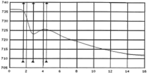
Another space of qualitative values can be defined by choosing <1><1 and taking integer multiples of <I> (i.e. { k <I> : k E Z } ) . However, Q· is has several advantages. First, x E Q41 can be arbitrarily small, while x E { k<l>} => lx I ~<I>. Thus, if <I> is too large, a small x may force a new choice of <I> and recomputing of all qualitative variables. Second, Q· is better for domains with variables on different scales where relative changes are important (e.g. see Figures 2a, 2b). In { k<l> }, choosing, say <I>= 0.01, to represent changes in a would imply a small rela tive change in u (e.g. from 735 to 730) maps to a large change in the qualitative space (e.g. 73500<1> to 73000<1>). Third, using Q· allows a natural definition of small relative changes as perturbations (see 3.1).
For QPA, Q· must be extended to intervals and more careful definitions of qualitative arithmetic are needed to ensure closure.
Definition: A qualitative interval label (QIL) is an interval of the form [ q 1 , q 2 ] where q 1 ~ q 2 , q1 E Qt and q2 E Qt.
Definition: The function qual(x) maps a real number x to the minimal QIL [ q l>q 2] such that q 1~ x ~q 2.
Definition: A QIL [ q 1 , q 2 ] represents a variable x if q1 ~X~ q2.
Definition: Two basic selector functions on QILs are qmin([q 1· q2]) = q 1· qmax([q I> q2]) = q2
Definition: The union and intersection of QILs are defined by
[q1,q2] U [q3,q4] = [min(q1,q3), max(q 2 ,q4)]
Notes: 1) Note that U and n can be easily general ized to more than two QILs.
2) As in [Davi-87], union is actually the convex hull.
Recently, [Simm-86] and [Will-88] have pointed out the need for algebras which combine quantitative and qualitative aspects. Both these works rely on real numbers and algebra for part of the representa tion task. QILs occupy an intermediate area, more quantitative than earlier systems (e.g. [Kuip-86] or [deKl-84]) and more qualitative than Q1 [Will-88] and the Quantity Lattice of [Simm-86].
The base <I> determines how the real numbers are partitioned. For a particular application, <I> can be chosen by analyzing the signals of a manoeuvre (e.g. examine initial values, relative magnitudes of peaks) If a higher resolution is needed, <I> can be changed dynamically (e.g. for <I>> 1, replace <I> by Y<t>). All QIL arithmetic can be performed exactly if <I> is a rational number or by simulating base <I> operations using integer exponents of <1>.
2.2 A QLM example
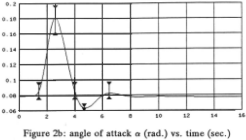
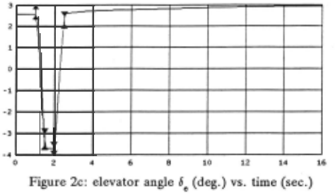
Figure 1 shows the equations of a linear model which applies to small motions in an aircraft's longi tudinal axes [Frie-85]. Figure 2 shows certain signals recorded during a "short period" manoeuvre, QILs representing the signals at critical points are super imposed on the signals in Figure 2 (QILs which would extend beyond the axes are drawn with an outward arrowhead). The segment from t = 1.0 seconds to t = 4.8 seconds is the most interesting. Selected gains for this segment are shown in Table 3 (to 2 significant decimal places) assuming <I> = 1.2.
This example is based on near-real-world data and will be referred to in the remainder of the paper.
2.3 Basic QIL arithmetic
Arithmetic on QILs, except for addition, follows the definitions of [Aief-83] and [Simm-86]. Q· is clearly closed under the operations X, ...;... and unary -, but not under the usual +· Thus it is necessary to define QIL addition, denoted by @, using the functions qual, qmin and qmax.
Definition: The sum of n QILs A 1 , ... , An is defined by
For example, [1,4] @ [2,8] = [qmin(qual(3)) , qmax(qual(12))] = [qmin([2,4]) , qmax([8,16])] [2,16].
Notes: 1) Most examples of QILs assume a base <I> = 2.
2) @ is not associative, for some QILs A, B, C, (A @B) @C ;eA @(B @C).
3) For any real x ,y, qual (x +Y) C qual (x) @qual (y).
Additive and multiplicative inverses do not, in general, exist in interval arithmetic.. Interval sub traction is defined in the obvious way:
However, using 8 leads to wide intervals (a possible loss of information). For example, [1, 4] 8 [1, 4] = [1, 4] @ [-4, -1] = [-4, 4]. This motivates the follow ing.
Definition: The function qdiff computes the differ ence between two QILs as
For example, qdiff([2,8],[1,4]) = [-4,-1] and [4,16] @ qdiff([4,16],[1,8]) = [-4,16].
Notes: 1) Clearly qdiff (A ,B) = [0, OJ <=> A = B 2) By treating intervals as sets of real numbers, as in [ Alef-83], it is easy to prove A @ qdiff (A ,B) ;:2 B.
2.4 Qualitative derivatives
A simplification typical of qualitative reasoning is that not all measured points of a signal are explicitly represented. An important decision is whether to represent time using intervals or a subset of meas ured points. The key problem is how to express the relation between consecutive qualitative values of a signal. In [Kuip-86], derivatives are known (either inc, std or dec) and all functions are "reasonable", therefore all transitions can be enumerated. Simi larly, [Forb-87] assumes the existence of a complete envisionment to predict future behaviours. In both cases filtering techniques are used to prune inconsistent behaviour sequences.
| Gain | Estimate | QIL |
|---|---|---|
| X u | -0.13 | [-0.13 '-0.11] |
| X 01 | -65.41 | [-66.25 '-55.21] |
| X e | 0.86 | [0.83 ' 1.00] |
| z u | -5.00e-5 | [-5.30e-5 , -4.42e-5] |
| z 01 | -0.65 | [-0.69 ' -0.58] |
| M 01 | -1.82 | [-2.07 ' -1.73] |
| M q | -1.26 | [-1.44 ' -1.20] |
| M e | -0.050 | [-0.054 ' -0.045] |
Derivatives. in QPA can be any value, therefore relations between consecutive values in a qualitative signals must be qualitative equations. For an inter val time representation , there is no apparent way to relate the values of signals and derivatives over an interval to their values over the next, or previous, interval. However, for a point-based representation, the derivative at a point can be defined in terms of adjacent points. Therefore, QPA uses the following definitions.
Definition: A signal x(t) is a sequence of N equally spaced measurements of x, x (t) <x 0, X , ··· , X >. T (N- 1)T
Definition: A qualitative signal is qx(t) = <(qxo,to), ... , (qxn ,tn-1) >, 0 =to< t1 < · · · < tn-1 = (N-1)7, some i, and qxj = qual(x; 7 ). a sequence where n<N, tj =iT -for
Definition: The derivative of a qualitative signal qx (t) at time t j is defined by qx j =
The derivative of qx is written as qx = <(qx 0,to) , ... , (qxn ,tn) >. Rewriting (2.1) gives constraints on consecutive values of a qualitative signal.
These constraints are used, for example, to force a(2.5) to be smaller (i.e. in the interval [0.13,0.16]). QPA must determine QILs for qa(2.0), qi:¥(2.0) and qa(2.5) which satisfy a derivative constraint of the form of (2.2) with qa(2.5) = [0.13,0.16].
Equation (2.2) is valid even though qx(t) does not necessarily represent the derivative of the real signal represented by qx(t). For example, in Figure 2a, the qualitative signals representing the state variable u has constant derivatives equal to [0, 0]. (In most cases tested, the qualitative derivative does in fact bound the real derivative.)
The points t 0 , t 1 , ··· , t n at which the qualita tive signal is defined are called cut-points. Cut points are chosen where the slope of x(t) changes (e.g. at maxima and minima) so that between cut points slopes are nearly constant. This ensures (2.1) will be a reasonable approximation to derivatives. The cut-points of a manoeuvre are the union of cut points of signals. A simple segmentation approximation algorithm is used to select cut-points (see [Pavl-73]). Table 4 shows the cut-points and qualitative representation for some of the signals of Figure 2, again with 2 significant digits and <I> = 1.2.
2.5 Interpreting QLMs as constraints
In QPA, QLM equations are interpreted as con straints on valid labels.
Definition: A constraint has the from <variable> = <expression>, where the expression involves only the operations EB' X ' u ' n·
Definition: A constraint is satisfied or consistent if the QIL resulting from evaluating the <expression> part contains the QIL labeling the <variable> part.
A QLM can be viewed as a network of constraints with two kinds of variables, basic and intermediate. Basic variables are those which can be measured or estimated, (i.e. gains, terms qual(t;-t;_1) and each qx j of a qualitative signal). Intermediate variables are computed by evaluating expressions containing only basic variables and previously computed inter mediate variables (e.g. qualitative derivatives).
When a QLM is initially computed, all constraints are consistent since the QIL labeling the <variable> is the result of evaluating the <expression> part. When variables in a QLM are modified (i.e. labeled with a different QIL) some constraints may become inconsistent. Re-establishing consistency in a QLM after some initial modifications is called a compensa tion problem.
3. Consistency after Perturbations
3.1 Perturbations of QILs
A perturbation is by definition a small change in a quantity. This is formalized for QILs as follows:
Definition: A perturbation P, ,s is a partial function from QILs to QILs determined by a pair of integers r , s . If [ q 1 , q 2 ] is a QIL then
Notes: 1) A perturbation may be undefined on some QILs, for example P 2, _ 1 ( [2, 8] ) is undefined.
2) A perturbation can never change the sign of an end-point of a QIL.
Definition: The order of a perturbation P, ,s is max ( I r I , Is I ) .
A compensation problem is defined by a QLM and a set of initial perturbations. QPA must solve the compensation problem by perturbing some of the remaining variables in the QLM. For example, with the signals of Figure 2 and Table 4, suppose the peak a(2.6) is too high relative to some measured reference. Then QP A could take the initial pertur bation P _1,_1( qa(2.6)) and try to find a solution consistent with the new label on qa(2.6).
| time | Q' | 8e |
|---|---|---|
| 1.0 | [0.065 ' 0.078] | [2.49 ' 2.99] |
| 1.4 | [0.078 ' 0.094] | [-2.49 ' -2.07] |
| 1.5 | [0.078 ' 0.094] | [-3.58 ' -2.99] |
| 2.0 | [0.13 ' 0.16] | [-4.30 ' -3.58] |
| 2.5 | [0.16 ' 0.19] | [2.07 ' 2.49] |
| 2.6 | [0.16 ' 0.19] | [2.49 ' 2.99] |
| 4.0 | [0.078 ' 0.094] | [2.49 ' 2.99] |
| 4.7 | [0.054 ' 0.065] | [2.49 ' 2.99] |
| 6.5 | [0.078 ' 0.094] | [2.49 ' 2.99] |
3.2 Consistency of individual constraints
A constraint is perturbed when a perturbation is applied to any variable in the constraint. For exam ple, [4,16) = [2,4) EB [4,8), but after P _1,_1 is applied to the left side, [2,8) ,e [2,4) EB [4,8). In QPA, com pensating a perturbed constraint means finding per turbations of other variables which re-establish con sistency. Completing the above example, P _1 _1([4,16]) = [2,8) = [1,4) EB [2,4) = P _1,0([2,4]) EB p -1:-1([4,8]).
There are a number of technical difficulties in compensating individual constraints. In particular, compensating addition and multiplication constraints can lead to multiple solutions (some heuristics can be used to reduce the. number of solutions). It is not necessary to discuss all the details, since there are deeper problems with propagating perturbations and an elegant approach to compensation which overcomes these problems.
3.3 Problems with compensation
Given a perturbed QLM, QPA must compensate all perturbed constraints to re-establish consistency. Compensation is a special case of interval propaga tion [Davi-87), since a perturbation re-labels a vari able with a new QIL. This suggests a control struc ture similar to the Waltz algorithm [Walt-75) could be used.
The Waltz algorithm is based on an operation, traditionally called REVISE, applied to a constraint C which removes any value v from the set of possi ble values of x if C cannot be satisfied with x = v. For some perturbations, compensation may have to enlarge a QIL (i.e. permit more values of x). Con sider the constraint [1,16) = [I/z,2) X [2,8), and sup pose the left side is fixed. A perturbation P0 _1( [2,8]) forces a compensation P0 1( [Ih,2]). Thus for compensation problems in QP A there is no analogue to the REVISE operation.
Several problems with using the Waltz algorithm to propagate intervals are analyzed in [Davi-87). In particular, for systems of constraints with linear relations the Waltz algorithm "tends to go into infin ite loops even for well behaved sets of constraints" [Davi-87, p. 305). Yet the constraints in a QLM are not at all well behaved, as they contain many loops. For example, in figure 1, a(t;) -+ q(t;) -+ q(t;) -+ a(t;) -+ a(t;), where -+ is read as "appears in a con straint with". Infinite loops are also possible if the starting state is inconsistent, which is precisely the case in a compensation problem. A problem inherent in interval arithmetic is the value of an expression depends on the order of evaluation of sub-expressions [Alef-83, ch. 3). Thus the order in which constraints are selected can affect the eventual solution and not just the running time.
3.4 Transformation to a CSP
A constraint satisfaction problem is specified by giv ing a set of variables, each with an associated domain, and a set of constraints. In QPA the con straints are the equations of the QLM and section 2.5 defines when a constraint is satisfied. The key idea in the transformation is to view QILs as atomic, not subject to modification during propagation. Then the domain of a variable is not its QIL, but the set of possible QILs with which it may be labeled during compensation. This transformation avoids the above mentioned problems with interval propa gation and permits QP A to use the consistency algo rithms of [Mack-77), [Mohr-86) and [Han-88). In particular, compensation cannot go into infinite loops since it is based on solving a finite CSP.
The important part of the transformation is defin ing the domain of each variable. In QPA there is a trade-off between the resolution Q·, the size of per turbations and the complexity of compensation. A finer discretization can be defined by setting <I> closer to 1, but then larger order perturbations may be required. This increases the complexity of com pensation, since there will be more solutions for a perturbed constraint.
When using QP A in a particular domain, the choice of the maximum order of perturbations must depend on <I>. Let Kb be the maximum order of a perturbation for a basic variable.
Definition: Let x be a basic variable labeled by A . Then x's compensation domain is
For intermediate variables, the definition of a compensation domain is problematic. Perturbations on inputs to a multiplication constraint could force a higher order perturbation as compensation on the output. A second constant K; ;::: Kb determines the order of perturbations allowed on intermediate vari ables.
Definition: Let y be an intermediate variable labeled by B. Then y's compensation domain is
The mapping from a compensation problem to a CSP, as defined so far, makes each compensation domain a set of QILs. To find consistent qualitative solutions for the compensation problem, the domains of basic variables which are initially per turbed are set to be exactly the perturbed QIL. This guarantees the solution of the CSP, if it exists, will include, and be consistent with, the perturbations input to QPA. In the CSP there is no distinction between input and output variables, therefore com pensating perturbations on outputs (i.e. reverse simulation) is no more difficult than solving for per turbed inputs. Network consistency algorithms use search to find consistent solutions. The possibility of multiple solutions, shows the possible trade-offs between different compensations. The solution of the CSP is the qualitative solution for QPA.
Finally, note that specifying the domain as a finite set of QILs would be impossible without a qualita tive (i.e. discretized) representation for endpoints.
4. Summary
4.1 Summary
This paper has presented the family of qualitative linear models, which is applicable to reasoning about dynamic systems with feedback and external control. QLMs are qualitative versions of first-order linear differential equations, as opposed to device centered models. An important problem when rea soning about dynamic systems is reasoning about perturbations. By using a qualitative interval label representation, perturbations to a system can be pre cisely defined. Since the QIL representation is qual itative, it is possible to reason about perturbations using network consistency algorithms whose com plexity is well known: Thus the qualitative represen tation avoids problems of propagating interval labels.
Most of QPA has been implemented and tested, including the basic qualitative calculus, operations on signals, and compensating perturbed constraints. Constraint satisfaction is presently implemented by a simple breadth-first search.
4.2 Future work
There are some areas for further research suggested by QPA and its application to dynamic systems. First, it would be interesting to extend QPA to more general differential equations. Second, the use of QPA in reasoning about discrepancies should be pursued. A possible analogy with mathematical optimization is under investigation, based on the idea of introducing perturbations to minimize discrepancies.
Acknowledgements
Important contributions to this work were made by Dr. Pierre Belanger of McGill University and Jonathan Levine of CRIM.
@inproceedings{ijcai1989p189,
  title     = {Perturbation Analysis with Qualitative Models},
  author    = {de Mori, Renato and Prager, Robert},
  booktitle = {Proceedings of the Eleventh International Joint Conference on
               Artificial Intelligence, {IJCAI-89}},
  publisher = {International Joint Conferences on Artificial Intelligence},
  editor    = {N. S. Sridharan},
  pages     = {1180--1185},
  year      = {1989},
  month     = {8},
  note      = {Knowledge Representation},
  url       = {https://ijcai.org/proceedings/1989/189},
}
TY - CPAPER TI - Perturbation Analysis with Qualitative Models AU - de Mori, Renato AU - Prager, Robert T2 - Proceedings of the Eleventh International Joint Conference on Artificial Intelligence, IJCAI-89 PB - International Joint Conferences on Artificial Intelligence PY - 1989 SP - 1180 EP - 1185 UR - https://ijcai.org/proceedings/1989/189 ER -Copied
Machine-readable versions of this paper, for tools and AI agents:





