
Diagnosing Temporal Misbehavior
Proceedings of the Twelfth International Joint Conference on Artificial Intelligence. Qualitative Reasoning. Pages 1116-1121.
© 1991 International Joint Conferences on Artificial Intelligence
Abstract
One of the main goals of model-based diagnosis is the detection and localization of failures that are very difficult to diagnose even for human experts. Especially transient failures require a sophisticated problem-solving strategy and often overcharge an experienced human diagnostician. Unfortunately, such transient failures occur in many applications and cause unacceptable misbehavior. Therefore, dealing with failures which have a temporal aspect is a challenging task for model-based diagnosis. However, current research on model-based diagnosis treats assumptions about the component behavior as static and therefore fails to reason about time-varying failures. In this paper we present a new approach to model-based diagnosis which enables us to deal with its temporal aspects.
- [Avizienis, 1982] Algirdas A vizienis. The four-universe information system model for the study of fault- tolerance. In 12th International Symposium on Fault- Tolerant Computing FTCS-12, pages 6-13. published by IEEE, June 1982.
- [Breuer, 1973] Melvin A. Breuer. Testing for intermit- tent faults in digital circuits. IEEE Transactions on Computers, C-22(3):241-246, March 1973.
- [Davis, 1984] Randall Davis. Diagnostic reasoning based on structure and behaviour. Artificial Intelli- gence, 24:347-410, 1984.
- [de Kleer and Williams, 1989] Johan de Kleer and Brian C. Williams. Diagnosis with behavioral modes. In 1122 Qualitative Reasoning Proceedings of the International Joint Conference on Artificial Intelligence (IJCAI), pages 1324-1330, De- troit, August 1989. IJCAI
- [de Kleer and Williams, 1990] Johan de Kleer and Brian C. Williams. Focusing the diagnosis engine. In First International Workshop on Principles of Diagnosis, Stanford, July 1990.
- [Friedrich and Nejdl, 1990] Gerhard Friedrich and Wolf- gang Nejdl. MOMO -Model-based diagnosis for everybody. In Proceedings of the IEEE Conference on Artificial Intelligence Applications (GAIA), Santa Barbara, March 1990.
- [Friedrich et al., 1990a] Gerhard Friedrich, Georg Gott- lob, and Wolfgang Nejdl. Physical impossibility in- stead of fault models. In Proceedings of the National Conference on Artificial Intelligence (AAAI), pages 331-336, Boston, August 1990.
- [Friedrich et al., 1990b] Gerhard Friedrich, Franz Lackinger, and Wolfgang Nejdl. Redefining the can- didate space in model-based diagnosis. In Proceedings of the European Conference on Artificial Intelligence (EGA/), pages 277-282, Stockholm, August 1990.
- [Genesereth, 1984] M. R. Genesereth. The use of design descriptions in automated diagnosis. Artificial Intel- ligence, 24:411-436, 1984.
- [Hamacher, 1991] Walter Hamacher. Modeling digital circuits for troubleshooting. Artificial Intelligence, 1991. to appear.
- [Kopetz, 1982] Hermann Kopetz. The failure fault (ff) model. In 12th International Symposium on Fault- Tolerant Computing FTCS-12, pages 14-17, June 1982.
- [Kuipers, 1986] Benjamin Kuipers. Qualitative simula- tion. Artificial Intelligence, 29:289-388, 1986.
- [Ng, 1990] Hwee Tou Ng. Model-based, multiple fault diagnosis of time-varying, continuous physical sys- tems. In Proceedings of the IEEE Conference on Ar- tificial Intelligence Applications (GAIA), pages 9--15. IEEE Computer Society Press, 1990.
- [Raiman et al., 1990] Olivier Raiman, Johan de Kleer, and Vijay Saraswat. Exploiting non intermittency. In First International Workshop on Principles of Diag- nosis, pages 120-123, Stanford, July 1990.
- [Reiter, 1987] Raymond Reiter. A theory of diagnosis from first principles. Artificial Intelligence, 32:57-95, 1987.
- [Struss and Dressler, 1989] Peter Struss and Oskar Dressler. Physical negation -Integrating fault mod- els into the general diagnostic engine. In Proceedings of the International Joint Conference on Artificial In- telligence (IJCAI), pages 1318-1323, Detroit, August 1989. IJCAI
References were extracted automatically from the PDF and may contain errors.
Full text extracted automatically from the PDF; figures, tables and equations may differ. The PDF is the version of record.
1 Introduction
Reasoning about behavioral abnormality of technical de vices is a key problem for model-based diagnosis. A lot of research work has already been done in this field which has typically concentrated on static devices and permanent abnormality (e.g. [Friedrich et al., _1990b; Davis, 1984]). Only recent approaches deal With the temporal aspects of abnormality (e.g. [Hamscher, 1991; Raiman et al., 1990]) .
Unfortunately, most practical applications require the ability of a diagnosis engine to detect and localize tran sient failures. Since the early days of fault-tolerant com puting most researchers in this field agree that diagnosis of transient failures is of crucial importance.
For example, [Breuer, 1973] writes
"Given that intermittents are tremendously more important to diagnose and that they do occur frequently, I propose that finding an or derly means to diagnose them is the most im portant unsolved problem in this area today."
In this paper we propose a framework for reasoning about the temporal aspect of misbehavior and therefore extend the traditional approach to model-based diagno sis. As a result, we are able to diagnose all types of failures including environmental disturbances as well as physical damages.
In Section 2 we start with a discussion of various prob lems of reasoning about temporal abnormality. Addi tionally, we give a clear distinction between failures and faults and classify them according to various properties. In Section 3 we present our framework of model-based diagnosis introducing failure intervals and temporal di agnoses. We introduce a probabilistic approach to as sign plausibility values to diagnoses w_hich is ~ased ~n the theory of Markov-processes in SectiOn 4. Fmally, m Section 5 we compare our framework to related research work in this field and present topics for future work.
2 Classifying Temporal Misbehavior
We start the discussion with the presentation of an ex ample which illustrates the problems of r~asoning abo~t various classes of faulty behavior and their causes. This discussion will lead us to the requirements which a model-based diagnosis engine has to fulfill if it is applied to time-varying systems.
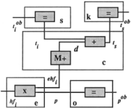
Consider a proportional-control heaterfcqoler [Ng, 1990]. This device consists of five components- the tem perature sensor s, the temperature control knob k, the power supply o, the electric heating/cooling component e and the proportional controller c. With respect to the difference (denoted with d) between the observed actual room temperature (tf 6 ) and the observed intended room temperature t~b (which is set by k), e generates heat flow hf,· which depending on the direction of the differ-· , d" ence can either be positive or negative. The a JUstment amo~nt is denoted with eh/;, the (observed) power input to the heater/cooler is denoted with (p 06 ) p.
Figure 1 shows the constraint model w~ich associat~s variables to components (we follow [Kmpers, 1986] m our terminology) :
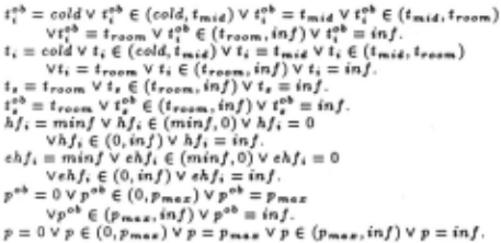
The qualitative quantity space for each variable is_ de picted in Table 1 (min/ < cold< tmid < troom < m/, min/< 0 < inf, 0 < Pma:c < in!).
In the following discussion we will use our example to discuss various scenarios of faulty behavior. We denote the qualitative system states as sets of qualitative pa rameter values and create a scenario as a sequence of system states. . .
We distinguish between faults from two VIewpomts using a temporal classification and a value classifica tion. Our terminology is closely related to the terms which have been used by the Fault-Tolerance commu nity as a standard for the last decade [Kopetz, 1982; Avizienis, 1982].
According to the distinction between failure and fault used by that community, we propose the notion fault to denote that the system's behavior deviates from the specification of correct behavior for some time interval. Note that the terms symptom and misbehavior, also used by the AI-Diagnosis community, are equivalent to our notion fault. The notion failure denotes the causes of faults. This distinction is important with respect to the temporal classification introduced in the following.
2.1 Temporal Classification
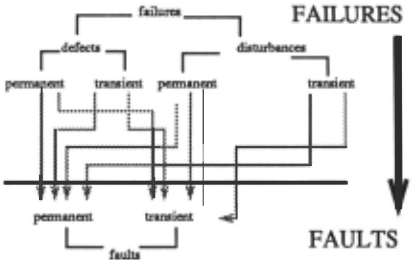
Figure 2 depicts the relation between failures and their possible manifestations (i.e. a failure can cause perma nent or transient faults). Nevertheless, failures need not necessarily alter the correct behavior during the mission of the system.
Failures have a temporal aspect and they do not nec essarily cause faulty behavior (e.g. their extent might be held locally by means of fault-tolerance). Conversely, every fault is caused by at least one failure. In order to distinguish between internal and external causes of faults, we introduce the notions defects for the former and disturbances for the latter. This distinction enables us to decide whether the system has to be repaired or the environmental conditions must be changed in the course of re-establishing correct behavior. Not also that the concept defect covers physical damages as well as design and assembling failures.
2.1.1 Permanent Faults
Let us assume that the proportional controller has a physical defect (e.g. component c exhibits a stuck-a t-O fault at d) . This defect exhibits the behavior pattern depicted in Table 2.
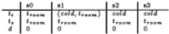
It is consistent to assume in state sO that the system behaves correctly. However, from state s1 to state s3, it is continuously inconsistent to assume that the system behaves correctly. The crucial property of a permanent fault is its permanent duration, not its beginning (i.e. a permanent fault can start during diagnosis).
Note that although the abnormal behavior is perma nent, its cause can be temporally limited (i.e. transient). For example, a temporal disturbance which changes the contents of a counter can cause a clock to behave con tinuously faulty.
2.1.2 Transient Faults
In order to introduce transient faults we discuss two examples in more detail. In addition to physical defects we present an example for an environmental disturbance because this type of failure is a prominent cause for tran sient faults.
Physical Defects: Let us now assume that a physical defect in the sensor causes a temporal deviation of the room temperature recorded by the sensor (t;) from the actual room temperature (tfb) (e.g. the response of the sensor is too slow due to an internal time delay) (see Table 3). Although the system shows transiently faulty behavior, its cause can permanently reside.

In contrast to permanent abnormality, this temporal deviation from the specified correct behavior is only vis ible for a finite period of time (during states s2 - s3). In state s4, however, the fault has disappeared, although the physical defect might still exist. Consequently, we can assume that the system behaves correctly in the states s4 and s5. Nevertheless, if we start with the same initial conditions we will get the same result (i.e. the fault is reproducible).
Environmental Disturbances: In the previous ex ample we have considered abnormality which can causally be explained by physical defects in the system.
However, each physical system works in an environ ment which influences its behavior in an unpredictable manner. For example, alpha particles can alter the state of memory cells. Temperature and humidity influence the correct behavior of electronic circuits.
From the viewpoint of repair, it is very important to distinguish between physical defects and environmental disturbances . The former have to be repaired, while the latter can only be tolerated in most cases. Therefore we have to include this distinction into our diagnosis process.
For example, consider the behavior pattern in Table 4.
| p Pmo:c pob Pma:c | 0 Pm•s Pm•z | Pm•z Pm•:c Pm•z |
This transient fault is caused by a temporary exter nal disturbance (e.g. the environmental temperature is too high) that results in a temporary shutdown of the power supply. Note that this fault is not caused by a component-oriented failure - only the observed behavior deviates from the desired. In fact, we have to concen trate on the causes of abnormality (e.g. physical defects or environmental disturbances) in order to repair.
2.2 Value Classification
In the above discussion we have assumed determinate faulty behavior. Determinate faults (also called stuck-at faults) do not show arbitrary behavior, the faulty behav ior is reproducible. More precisely, determinate behavior is characterized by a functional relation between the ex ogenous and the endogenous variables of the system.
Unfortunately, some failures do not cause determinate behavior. In this sense, the impact of an alpha particle on a counter produces indeterminate, transiently faulty behavior. For example, let us assume the following two behavior patterns of the heater/cooler that are depicted in Table 5 (state sN denotes a possible successor state of sO).
This indeterminate fault is caused by a loose cable in the sensor display which produces different values of resistance. Note that these behavior patterns are only two examples from a set of possible faults resulting from this failure.
| sO | sN |
|---|---|
| trocnn cold | |
| troom tmid |
2.3 Requirements for Temporal Diagnosis
From the above discussion we derive the following con clusions and requirements for reasoning about temporal abnormality. These requirements serve as a guideline for our approach to model-based temporal diagnosis.
In order to distinguish between temporal properties of failures we have to model them explicitly. This is due to the fact that we can not draw conclusions about the temporal nature of failures by solely considering the tem poral properties of their manifestations (i.e. the faults). For example, transient faults can be caused by perma nent and transient failures both.
It is not sufficient to distinguish between determi nate and indeterminate behavior of components for mak ing assumptions about permanent and transient behav ior (i.e. intermittent, according to the terminology of [Raiman et al., 1990]). We rather have to reason about the possible transitions between different combinations of failures. This view enables us to distinguish between the different classes of failures with a finer temporal granularity and leads to an enhanced characterization of the assumptions about the system's history and its present state (i.e. diagnoses).
The operation of every device depends significantly on its environmental conditions. Consequently, we have to include the environment in our models to be able to reason about it. This is a necessary presupposition to distinguish between various causes for faulty behavior (i.e. defects and disturbances).
3 Defining Failures and Temporal Diagnoses
Continuing the above discussion, we present our new ap proach to model-based temporal diagnosis.
We start with a formal definition of failures and their temporal properties. Furthermore, we extend the tradi tional notion of a diagnosis with respect to these prop erties and introduce temporal diagnoses.
3.1 Failures
Faults represent the abnormal behavior of components and systems, whereas failures are the causes of such ab normal behaviors.
Definition 1 (Failures) F AI is a finite set of constants representing failures.
The set of possible failures for a component c is de noted by F AI( c). A failure is associated with a compo.. nent c at time instance t by the predicate failure, e.g. failure( c, shorted)t . This association allows a classifi cation which is valid for a broad range of failures. Nev ertheless, we do not treat this association as a necessary presupposition but rather as an aid.
Consequently, we distinguish between component dependent failures, which we denote defects, and component-independent failures which we call distur bances.
Note that a failure may not be in contradiction with the correct behavior and that assuming a component to be associated with several failures at time point t is valid. For example, ...,ab( c) 1\ failure( c, outpuLshorted)t as well as failure( c, outpuLshorted)t 1\ failure( c, input_shorted)t are no contradictions (-,ab(c) denotes the correct behavior of component c).
This discussion leads us to the notion failure behav ior.1
Definition 2 (Failure Behavior) The behavior of a fail ure f E F AI for an entity c E COM PSis a set of First Order-Sentences B , such that "'T: failure(c,J)T- B .
According to this definition, a fault can be character ized by several failure behaviors. [Hamacher, 1991] in troduces the concept of a syndrome which denotes sets of failures having the same behavior. This concept reduces the complexity of the diagnosis process since the num ber of failures can be significantly diminished. This idea can easily be integrated into our framework by viewing a syndrome as an abstract failure.
In contrast to related approaches which are based on behavioral component modes, we view the central goal of model-based diagnosis to identify failures. Consequently our concept of a temporal diagnosis, as defined later, will be a set of assumptions about the existence and absence of failures. ·
Similar to the unknown fault mode of [de Kleer and Williams, 1989; Struss and Dressler, 1989] we include un known failures if the failure description is not complete.
3.1.1 Temporal Classification
We distinguish between permanent and transient fail ures to make a first qualitative distinction between dif ferent levels of plausibility.
In order to define temporal diagnoses we have to ex press temporal properties of failures. We therefore define failure intervals as follows. Let in(T, Sets) be an abbre viation for V,eset. T E s.
Definition 3 (Failure Intervals) INTFAI(c,f) is the fi nite set of closed time intervals for a entity c E COM PS and a failure f E F AI such that
1 In the following SD,COMPS, and OBS are defined as usually (e.g. [Reiter, 1987]). However, COM PSis extended in order to include constants representing the environment, the design, etc., in addition to device components. There fore we rather talk about entities than about components. Additionally, SD and OBS may be time-varying.
- For each pair of different intervals [At, Et], [A2, .&.2] the relation holds that one interval is before the other, i.e.
- Entity c is assumed to have failure f :
'v'At.Et,A2,E2: [At,Ed EINTFAI(c,f)l\
[A2, E2] E INTF AI(c,f)l\ [At, El] #- [A2, E2] _. 3t : (Et < t < A2)V (E2<t<A1).
'v'T: in(T,INTFAI(c,f)) ..... failure(c,f)r.
The sentence "'T: in(T, I NTF AI(c, f))+-+ failure(c , f)T expresses that at all time points which are included in an interval i E I NT F AI( c, f) the component c has failure f. At all time points which are in no failure in terval for f the component c does not have failure f . If we want to express that a component c does not have failure I then I NTF AI(c, f)= {0}.
For example, INTFAI(r1 ,shorted) = {[tl,t2), [t3, t4]} has the meaning that entity r 1 has the failure shorted exactly in the time intervals [tl, t2) and [t3, t4].
According to the above discussion, we formalize the notions of permanent and transient failure.
Permanent Failures: Permanent failures are irre versible changes in components, such as shorted tran sistors or continuous environmental disturbances. They lead to a permanent transformation of the original sys tem into a new system that has a different description and will not always behave in the proper manner.
Let t0 be the time point when the system has fulfilled its purpose and ta be the opening of operations of the system (i.e. the birth of the system).
Definition 4 (Permanent Failure) A failure f E F AI for a component c E COM PS and a relevant inter val [ta, to) is permanent starting with tb iff there ex ists a time interval [tb, te) E I NT F AI( c, f) such that tb $to $ te.
Transient Failures: The attribute transient is as signed to a failure which resides only temporarily in the system, but which can nevertheless cause permanent faults. An obvious cause of such faults is external in terference of short duration, for example, the impact of an alpha particle on a memory cell. Another cause for a temporary deviation of component variables are tem perature variation or delays in timing caused by stray capacitance.
Definition 5 (Transient Failure) A failure I E F AI for a component c E COM P S and the relevant inter val [ta, to] is transient iff there exists a time interval [tb,te] E INTFAI(c,f) such that te <to.
Note that these definitions cover a broad range of pos sible combinations of failures. For example, we are able to represent the frequent case that transient failures can start to be permanent later.
3.2 Temporal Diagnosis
According to the above concepts we define a temporal diagnasis as follows. Let FS = {(c, f)lc E COM PS, / E FAI(c)} .
Definition 6 (Temporal Diagnosis) A temporal diagno sis ~ for a relevant interval (ta, tn] is a set of triples {(c, f, INTFAI(c,f))i (c,f) E FS} for (SD, COMPS, OBS, F AI) such that
is satisfiable.
A temporal diagnosis assigns to each failure (which is associated to an entity) a set of failure intervals, such that, with respect to the relevant interval, in these failure intervals the failure is present and at all time points not covered by these intervals the failure is not present.
This definition of a temporal diagnosis includes all consistent assumptions about possible occurrences of failure combinations. Furthermore, the concept of a tem poral diagnosis is general enough to allow the application of general theorem provers for consistency check (e.g. [Friedrich and Nejdl, 1990]).
We can apply various criteria how to assign plausi bility values to the diagnoses. In Section 4 we present techniques for the computation of such plausibility val ues based on the failure rate A and the repair rate J.l.
Note that we do not need a temporal classification of behavior (i.e. faults) for temporal diagnosis because we can derive faults from failures. For a given tempo ral diagnosis we are able to predict this faulty behavior weighted with a plausibility value.
As a result, we have achieved a straightforward gener alization of the traditional view of diagnosis by adding a temporal dimension to the candidate space (i.e. diag nosis lattice).
4 Ranking of Temporal Diagnoses
We can distinguish between various criteria for the plau sibility of a diagnosis. The most popular ones are either the minimal or irreducible or most probable sets of as sumptions about the behavior of components.
The diagnosis process as introduced by [de Kleer and Williams, 1989] generates the set of most probable (lead ing) diagnoses . The different modes of behavior of the components are weighted by a static a priori probability value. It is assumed that components are in a specific mode of behavior and do not switch between various modes during diagnosis. The a posteriori probabilities are computed for these diagnoses in order to rank them and to select the best next measurement point.
If, however, we include time into diagnosis we have to allow transitions between states when failures exist and when they have vanished.
We therefore propose the use of an appropriate statis tical model using Markov-processes to compute proba bilities of temporal diagnoses.
4.1 Statistical Model
We presuppose that failures are independent. Further more, time is assumed to be linear and discrete and will be represented by natural numbers.
Let P,(t) denote a probabilistic function (P,(to) = 1, P1(oo) = 0) where P1(t) is the probability that failure f is not present in the system until time point t.
Let further d1(t) denote the failure density function for failure f with
We define the failure rate AJ(t) for failure f as
Based on a probabilistic function MJ(t) which ex presses the probability that failure f has been repaired until time point t, the repair rate J.lJ(t) is defined anal ogou.sly to AJ(t) . J.lJ(t) covers self-repair and external repair.
For many failures P1 (t) and MJ (t) will be exponential functions and therefore result in a constant failure rate and repair rate. This is valid for most systems during the main part of their life cycle, excluding short time intervals after the start and before the end of the opera tion. Therefore, we assume both A and J.l to be constant in the further discussion.
In the following we show how to compute the statistics of temporal diagnoses using Markov processes. In our approach, each state of a Markov process represents a set of assumptions about the presence or absence of each failure f E F AI. The transition arc between two nodes represents one discrete step from time point t; to time point ti+I·
4.2 Computation
Let .6. be an element from the set of temporal diagnoses and let f E F AI be a failure. Let t0 be a time point where no failure is present in the system (i.e. to = ta)· Consequently, the initial probability at time point to that f is not present is 1. In order to compute the prob abilities for a temporal diagnosis at time point tn (i.e. tn = to), the following computation step has to be ap plied to all time points t; for i = 1, ... , n.
The temporal diagnosis .6. defines for each time point t; a partition ofF AI into the two disjunct subsets F AlP and F AI". FA If ( F AI~) denotes the set of failures which are assumed to be present (absent) at time point t;.
We distinguish between four types of transitions be tween time point t; and t;+I. Pt; ( .6.) denotes the actual probability of .6. at time point t;.
We compute Pti+l as follows:
- fail transition: for each failure f E F AI~ and f E FAif'+,: Pt;+· (.6.) := Pt;+l (.6.) X AJ
- no-fail transition: for each failure f E F Alf and f E FAI~+~: ' Pt·+· (.6.) := Pt·+· (.6.) x (1- AJ)
- repair transition: for each failure f E F Alf, and f E FAI~+,: Pt;+1 (.6.) := Pt;+1 (.6.) X J.lJ
- no-repair transition: for each failure I E F Aif; and I E F Aifi+·:
In order to normalize the probabilities of all temporal diagnoses with respect to the interval [to, t;], we divide their probabilities by the sum of the probabilities of all temporal diagnoses in [to, t;] .
However , for realistic applications the large number of possible diagnoses will prevent the computation of the normalization. As noted by [de Kleer and Williams, 1990], this normalization does not affect the ranking of the diagnoses.
In model-based diagnosis, we distinguish between diagnoses which explain the observations, and diag noses which do not constrain the possible outcome of a probe. From a rational point of view, such observation explaining diagnoses are more plausible and therefore preferred. In [de Kleer and Williams, 1990], the proba bilities of these diagnoses are unchanged, while the prob abilities of not explaining diagnoses are divided by the number of possible outcomes of the probe. In particular, the concept of explanation is related to the outcome of the next probe. The value that expresses the capabil ity of a diagnosis to explain outputs (i.e. endogenous) is only recomputed if additional inputs (i.e. exogenous) are selected and measured.
Similar to [de Kleer and Williams, 1990], we use Bayes' rule to compute the posterior probability of a temporal diagnosis and also assume that the set of possible out comes of a probe is finite. We extend the heuristic of [de Kleer and Williams, 1990] to weight the explanational capabilities of a temporal diagnosis:
Each temporal diagnosis divides OBS into the two disjunct subsets 0 B Sen (denoting endogenous observa tions) and OBSe:c (denoting exogenous observations). We only have to consider the explanational capability of temporal diagnoses with respect to OBSen, because exogenous observations can only be explained by the en vironment.
For each obs E 0 BSen of ·a temporal diagnosis .6. we weight the probability Pt .. (.6.) as follows :
where m00, is the number of possible outcomes of a probe which has been observed to be obs.
4.3 Example
In this section we show how our approach applies to the example of Section 2.
We consider the subsystem that consists of the power supply o and the heating/cooling component e. Con sequently, we observe the two endogenous variables p and hi; (the exogenous variables are (p 00 = Pma:c)T and (ehl; = (0, inf))T for all T 2:: tl).
As an example, two possible failures are included:
with AJ 0 = 1 X lQ- 2 , AJ. = 1 X 1Q- 2 ,J.l/o = 1 X 10- 5 , J.lJ. = 1 x 10- 5 .
The history of the system, containing the endogenous observations and the weighted transitions, is depicted in Figure 3 (/0 (!.) means this failure is in the system). As stated above, we assume that at time point to no failure is present in the system.
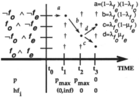
In Figure 3, bullets denote the nodes of the Markov process while daggers denote combinations of failure as sumptions that are not in any temporal diagnosis.
Table 6 depicts the weighted temporal diagnoses (not normalized, both diagnoses are explaining).
| TRANS. | DIAGNOSES | PROB.• |
| (a , b, e) | (( o, J o• [ta, tal), ( e, J., [t2 , ta))) | 9.6 X 10- |
| (a, b, d) "probability | ((o, /o , [ta, tal) , (e, /., [t2, t21)) not normalized | 9.7 x to-to |
The first diagnosis in Table 6 is more likely since the probability that failure 1. is persistent is higher than the probability of its repair.
5 Related Work
Beside others, there are at least two remarkable papers (i.e. [Genesereth, 1984] and [Raiman et a/. , 1990]) deal ing with transient (intermittent) behavior. In the ter minology of [Raiman et a/., 1990], a component behaves non-intermittently if its outputs are a function of its in puts, e.g. the additional axiom for an or-gate is:
where F represents an unspecified function.
Since the temporal aspect of the faulty behavior of components is not represented, the only achievable state ment about defect components is whether they behave intermittently or not, no matter whether the current be havior status is correct or abnormal. Clearly, one of our goals is to express exactly when the system behaves cor rectly and abnormally.
In order to use non-intermittency axioms the non intermittent behavior (correct or faulty) has to be func tional. Consequently, the general I/O-behavior has to be modeled functionally even for permanent failures which is a severe restriction of generality. If we introduce such non-intermittency axioms, random number generators have intermittent behavior, for example.
There are some other important papers extending static diagnosis (i.e. [Hamacher, 1991]). Their work fo cuses on dealing efficiently with temporal system descrip tions and considers the assumptions about failures as permanent whereas our aim is to deal with the temporal properties of diagnoses.
6 Conclusions and Future Work
We have presented a new framework for model-based di agnosis which overcomes many of the current limitations. The distinction between failures and faults and their classification according to time and value has proven to be important in the course of diagnosing time-varying systems.
We have introduced temporal diagnoses as a general ization of the traditional notion of a diagnosis by a tem poral aspect. This generalization enables us to detect and localize permanent and transient failures.
Furthermore, we have presented a probabilistic ap proach using Markov-processes to assign plausibility val ues to temporal diagnoses. The use of Markov-processes allows us to include failure - and repair - rates and to evaluate all types of transitions between possible failure states.
We are currently investigating various search tech niques (heuristic) for plausible temporal diagnoses using physical impossibility [Friedrich et al., 1990a] as one of several pruning techniques. The problem of finding the most plausible diagnoses is one of the most challenging and open problems in current model-based diagnosis re search.
Acknowledgements
The contents of this paper have benefited from discus sions with Anton Beschta, Oskar Dressler, Hartmut Frei tag, Michael Montag, and Peter Struss.
@inproceedings{ijcai1991p164,
  title     = {Diagnosing Temporal Misbehavior},
  author    = {Friedrich, Gerhard and Lackinger, Franz},
  booktitle = {Proceedings of the Twelfth International Joint Conference on
               Artificial Intelligence, {IJCAI-91}},
  publisher = {International Joint Conferences on Artificial Intelligence},
  editor    = {John Mylopoulos and Ray Reiter},
  pages     = {1116--1121},
  year      = {1991},
  month     = {8},
  note      = {Qualitative Reasoning},
  url       = {https://ijcai.org/proceedings/1991/164},
}
TY - CPAPER TI - Diagnosing Temporal Misbehavior AU - Friedrich, Gerhard AU - Lackinger, Franz T2 - Proceedings of the Twelfth International Joint Conference on Artificial Intelligence, IJCAI-91 PB - International Joint Conferences on Artificial Intelligence PY - 1991 SP - 1116 EP - 1121 UR - https://ijcai.org/proceedings/1991/164 ER -Copied
Machine-readable versions of this paper, for tools and AI agents:





