
When Oscillators Stop Oscillating
Proceedings of the Twelfth International Joint Conference on Artificial Intelligence. Qualitative Reasoning. Pages 1109-1114.
© 1991 International Joint Conferences on Artificial Intelligence
Abstract
Diagnosing analog systems, i.e . systems for which physical quantities vary over time in a continuous range is , in itself, a difficult problem. Analog electronic circuits, especially those with feedback loops, raise new difficulties. Oscillators, a special case of such circuits, are even more difficult to diagnose. This is because most faults lead to the same type of symptom: the oscillator just stops oscillating, the different electric signals remaining hopelessly flat! This paper shows how a program implementing a model-based diagnosis theory can be used to diagnose oscillators. We frrst present CATS, an ATMS-Iike domainindependent conflict rccognthon engine, adapted for diagnosing continuous timevarying physical systems. Its original feature is that it works on data that arc arrays of numeric intervals so as to deal with values that change with time ·and are inaccurate. ll1cn we show how to use this program for diagnosing oscillators, pointing out the advantage of using external stimulation. Experimental results arc given through the example of an astable multivibrator.
- J.S. Brown, R .R. Burton, and J. de Kleer, "Pedagog- ical, Natural Language and Knowledge Engi- neering Techniques in SOPHIE I, II and Ill," Intelligent Tutoring Sy.rtem.r, Academic Press, 1982.
- P. Dague, P. Deves, P. Luciani, and P. Taillibert, "Analog Systems Diagnosis," Proceedings of the Ninth ECA/, Stockholm, August 1990a.
- P. Dague, P. Devcs, and 0 . Raiman, "Trouble- shooting: when Modeling is the Trouble," Pro- ceedings of AAAI Conference, Seattle, July 1987.
- P. Dague, 0. Jehl, and P. Taillibert, "An Interval Propagation and Conflict Recognition Engine for Diagnosing Continuous Dynamic Systems," Lecture Note.r in Artificial Intelli- gence, vol. 462, Springer-Verlag, Vienna, Sep- tember 1990b.
- E. Davis, "Constraint Propagation with Interval Labels," Artificial Intelligence 32, 1987.
- J. de Kleer, "An Assumption-based TMS," Artificial Intelligence 28, 1986.
- J. de Klecr and B.C. Williams, "Diagnosing Multiple Faults," Artificial Intelligence 32, 1987. .
- J. de Klecr and B.C. Williams, "Diagnosis wtth Behavioral Modes," Proceedings of the Elev- enth IJCAI, Detroit, August 1989.
- W. Ilamscher, "Temporally Coarse Representat~on of Behavior for Model-based Troubleshootmg of Digital Circuits," Proceeding.r of the Eleventh /JCAI, Detroit, August 1989.
- W. llamscher, "XDE: Diagnosing Devices with Hierarchic Structure and Known Component Failure Modes," Proceeding.r of the Sixth IEEE Conference on A I Application.r, Santa Barbara, March 1990.
- R.-W. Liu, selected papers on Analog Fault Diagno.ris Advances in Circuits and Systems, IEEE Press, 1987.
- G . Loveday, Electronic Te.rting and Fault Diagno.ris, Second edition Longman Scientific and Tech- nical, 1989.
- R . Moore, Interval Analy.ris Series in Automatic Com- putation, Prentice-flail, 1966.
- II.T. Ng, "Model-based Multiple Fault Diagnosis of Time Varying, Continuous Physical Devices," Proceedings of the Sixth IEEE Conference on A I Application.r, Santa Barbara, March 1990.
- Y. Pan, "Qualitative reasoning with deep-level me_ch- anism models for diagnoses of mecharusm failures," Proceeding.r of the First IEEE Con- ference on AI Applications, Denver, 1984.
- Raiman, "A Circumscribed Diagnosis Engine, " Lecture Notes in Artificial Intelligence, vol. 462, Springer-Verlag, Vienna, September 1990.
- R. Reiter, "A Theory of Diagnosis from first Principles," Artificial Intelligence 32, 1987.
- K . Siet7.ega and R. Rastogi, "Model-based reasonning finds Analog PCB faults," Electronics Test, pp. 26-30, March 1990.
- P. Struss and 0. Dressler, "Physical Negation -Inte- grating Fault Models into the General Diag- nostic Engine," Proceeding.r of the Eleventh JJCA/, Detroit, August 1989. IJCAI
- B. C. Williams, "Doing Time: Putting Qualitative Rea- soning on Firmer Ground," Proceedings of AAAI Conference, Philadelphia, August 1986.
References were extracted automatically from the PDF and may contain errors.
Full text extracted automatically from the PDF; figures, tables and equations may differ. The PDF is the version of record.
1 Introduction
In additi<>n to pure analog circuits, the increasing usage of analog/digital hybrid circuits and the recognition of the importance of "analog" faults in digital circuits makes analog fault diagnosis ever more important. Unfortunately this raises many specific problems:
- There is a continuum of possible failures because of the continuous character of the parameters of such cir cuits, whereas for digital circuits a large percentage of faults can be modeled by stuck-at-one faults and stuck-at-zero faults.
Philippe Deves, Pierre Luciani, Patrick Taillibert
Dassault Elcctronique 55 quai Marcel Dassault 92214 St Cloud- France
- Both measurements and component parameters are inaccurate.
- Not even 50% of the measurements can be taken (voltages but not currents).
- A faulty component can provoke other components to shift well away from their nominal behavior and yet be correct.
- Complex feedback structures arc encountered. The effects of a fault propagate around loops, making it impossible to use conventional diagnostic techniques which try to track fault effect backward to a single component. Breaking the loop (as is often proposed in repair manuals [Loveday, 1989]) is impossible in a large number of cases since, in addition to the prac tical problems that would arise, it would require the elaboration of a replacement signal so as to avoid pushing the circuit towards an unacceptable state of behavior.
- Multiple faults are not a rare occurrence, since the failure of one component can have a knock-on effect on others.
The consequence of these difficulties is that the kind of orute force"' fault simulation classically used for diagnosing digital circuits is unrealistic for analog cir cuits. Only partial solutions have been obtained in this way [Liu, 1987].
Some of these difficulties are naturally overcome by using the general model-based diagnostic framework [de Klcer and Williams, 1987, Reiter, 1987], which allows diagnosis based exclusively on the description of the structure of the circuit, the models of correct behavior of its components (possibly extended to include faulty behavior) along with the assumptions governing the validity of these models and, lastly, the observation (measurements). The central task of diag nosis is thus to detect discrepancies between predicted behavior (from models) and observation and to build the corresponding minimal conflicts, i.e. minimal sets of assumptions which support a discrepancy. This task is classically carried out by coupling a predictive engine with an /\TMS [de Klccr, 1986]. The diagnoses, i.e.
all sets of component behavioral modes that are con sistent with current measurements, arc then computed from the conflicts.
However, this approach docs not tackle certain diffi culties specific to analog circuits, i.e. modeling, and inaccuracy and time management. This explains why most of the model-based diagnostic systems (GDE [de Kleer and Williams, 1987], SHERLOCK [de Kleer and Williams, 1989], GDE+ [Struss and Dressler, 1989], X DE [Ilamschcr, 1990]) arc in fact applied only to digital circuits. Only a few systems have been designed for analog circuits (SOPIIIE [Brown et al., 1982], DEDALE [Dague et al., 1987], ELECTRA [Sierzega and Rastogi, 1990]), but they propose only partial solutions.
In [Dague et at., 1990a], we have recently presented a system for applying model-based diagnosis to analog circuits and begun to experiment them. Continuing with this investigation we show in section 3 of this paper that our solutions also apply to the special case of oscillators (circuits without input and containing a positive feedback loop) in spite of specific difficulties . Through experiments we show that the use of external stimulation is a good way to reduce the ambiguity of the diagnoses obtained by our program. But before hand, in section 2, we describe the domain independent conflict recognition engine (CATS) used by our program. CATS has been specially designed to reason on arrays of intervals representing continuous time-varying signals. This algorithm allows the cou pling of an extended A TMS incorporating the interval semantics with any given interval computation primi tive, in such a way as to focus on the detection of nogoods. It also reduces the cost of label propagation by recording only one label for an array of intervals.
2 Conflict Recognition
CATS is a domain-independent conflict recognition engine for diagnosing continuous dynamic physical systems. It receives as input both constraints under assumptions coming from the structure and the models, and values coming from measurements; it produces as output all the minimal inconsistent sets of assumptions (bearing in mind that this completeness is defined w.r.t. a given modeling and numenc propa gation, both incomplete in essence) .
2.1 Representation of Physical Quantities
We have to deal both with physical quantities, the values of which change over time in a continuous range and are inaccurate, and with the unavoidabk imprecision of modeling. In DEDAJ ,E [Dague et at., 1987] we used qualitative modeling in terms of relative orders of magnjtude, since only direct voltages were measured and thus all the quantities were constant over time. Consequently, only failures observable in direct mode could be diagnosed. We are now inter ested in circuits where the important region of behavior of the components is when they behave dynamically. A qualitative scale cannot be used to detect fast variations and thus to detect subtle discrep ancies (it often happens that discrepancies occur over a very short period of time). It is the reason why we have decided to represent inaccuracy upon values (of either a quantity at a given instant or a parameter of a model) by an interval, which is computed by takjng into account the precision of the measuring device or of the modeling.
We have rejected the idea of using an interval repre sentation of time and of expressing quantities in terms of their concise histories made up of episodes, i.e. maximal time intervals during whlch the (interval) value of the quantity remains constant. Although this is used by temporal propagators such as TCP [Williams, 1986] and TINT [Jiamscher, 1989] for discretely modeled systems (e.g. XDE uses TINT for troubleshooting digital circuits), it seems difficult to transpose to continuous systems. Pirstly, since it is rare to obtain the same interval value at two different instants, defining episodes is not simple. Secondly, even if such a representation could be obtained, it would rapidly become useless since computations on values are performed to predict others, using models. Indeed, during a given time interval of observation, the regions where different quantities vary very quickly (corresponding to very small episodes) or vary very slowly (corresponding to large episodes, whlch are interesting from the point of view of conciseness of information) would be different from one quantity to another. Simply adding two quantities might lead to a new partition in very small episodes. What we would end up with is a kind of fine sampling for a lot of quantities, except that the samples would not coincide!
We have thus decided, in contrast with [Pan, 1984, Ng, 1990], to rely upon a proper sampling pro cedure. Every value of a quantity is represented by an array of numeric intervals, where each interval expresses the value at the corresponding sample. It is accompanied by a triplet defining the start instant, the sampling increment and the number of samples. During a sequential measurement process the sampling increment and the number of samples are generally kept constant and it is assumed that measurements can he repeated in such a way that start instants can be synchronized: comparison of values or computation on values is thus possible.
The most general form for an input of CATS is: x 1 , ······· , xk :::. x where each antecedent Xj of the left -hand side conjunction (possibly empty) and the consequent x are either propositional assumptions or constraints (equalities or inequalities) on given quanti ties. For example, the model of a capacitor c with I 0 ILF ± 10% capacitance and accesses a and b is:
correct(c) ~
i_c_a = [9.E-6,11.E-6] x derivative(v_c_a_b)
Part of the model of a transistor t with a gain ranging from 50 to 200 is:
correct(t) ~ i t c ~ -l.E-4 correct(t),v_t_b_e ~ 0.6, v_t_c_e ~ 0.3
~ i_t_c = [50,200] x i_t_b
The structural constraints which declare that access a of component c is linked to access k of node n are: v_c_a = v_n_k, i_c_a = -i_n_k
A value resulting from a measurement is:
v_rl_a_b = ([2,2.2],[2.5,2.8],[2.9,3.4]) All this input may be given incrementally.
2.2 Interval Propagation and Conflict Recognition
For reasons of clarity we consider here the problems that arise with continuous quiescent quantities whose values are intervals; temporal aspects will be examined later.
2.2.1 Semantics of the Data
A datum is a pair (q,i) where q is the name of a quan tity and i a numeric interval, meaning that the value of q belongs to i. The set of all computed values of a given quantity q is thus partially ordered by the inclu sion of intervals.
The semantics of intervals is expressed by the three following first-order interval rules, which are needed to ftre propagation and detect discrepancies. For example, given 3 data (Q1,[0,4]), (q1,(3,6]), (q2,[4,8]) and one input rule provided by a constraint (Q1,[2,5J)~(Q2 1 [1,3]), we have to use successively:
· the intersection rule (Q, I!)' (Q' 12 )1-+ (Q' I I nl2) which builds the new datum (q1,[3,4]).
· the inclusion rule
(Q, I 1), (Q 1 12), I 1CI2~-+{ (Q, I 1) ~ (Q, 12)) which records the justification ( q 1 , [3, 4]) ~ ( q 1, [2, 5]), needed to ftre the input rule in order to deduce the datum ( q2, [1, 3]).
· the falsity rule (Q,Iil)~-+.l which, after reapplying the intersection rule to (q2,[1,3]) and (q2,[4,8]) to build ( q 2 , lil) , detects a discrepancy.
2.2.2 Interval Propagation
CATS uses the classical interval propagation tech niques already found in [Brown ct al., 1982] and described by [Davis, 1987]. In practice CATS may usc any interval refmement computation primitive which is sound and also monotonic w.r.t. interval inclusion.
Soundness means that the computed interval of a given quantity always contains all possible values of this quantity. Although this theoretical domain of values is usually an interval (because the constraints arc usually expressed as continuous piecewise linear functions), it is generally impossible to compute it exactly (see [Moore, 1966] for mathematical aspects of interval calculus), i.e. the propagation procedure is not complete. For example, a naive propagation of interval i through the function y=x+ 1/x according to the formula i+1/i gives for i=[0.5,2] the interval [1,4] which is larger than the exact result [2, 2. 5]. When the domain is not an interval, but can yet be com puted, we nevertheless enlarge it to an interval. For example, dividing by zero is not continuous and would lead to a disjunction of intervals that is too complex to manage. 1/[ -1,2] = ]-«>1 -1] U [0.5,t<JO( is thus enlarged to )-«>, + aof.
Monotonicity (w.r.t. interval inclusion), which is obviously theoretically true for continuous functions, is also true in practice when classical propagation proce dures are used.
Any input of CATS such as f ( q 1 ' , ·· 1 qm') ~0 ~ c ( q 1 1 ···· 1 qn) is expressed as predictive ftrst-order rules on data:
{QI,II), ·. ,(qn,In) 1-+ (Qk 1£k{II, .... ,In)), where f and each ~t are the computation primitives associated with function f and constraint c.
A problem of interval refinement is that it may go into an infinite loop [Davis, 1987]. To prevent this, a halt condition is required. It is defined by the following qualitative equality between intervals using two thresh olds A and~::
[a,b]:::::: [max(a,-A),min(b,A)]
[a 1b] :::::: [c,d] if la-cl + lb-dl < E Considering the way floating numbers are represented in a computer, this halt condition is satisfied in prac tice. Moreover A and t: have physical counterparts: the upper bound for a value of a physical quantity can be known as a property of the artifact and the lower hound rc~mlts from the imprecision of both measure ment and modeling. In this sense, this halt condition ensures a wcomputationally and physically complete" saturation.
2.2.3 Interval Semantics and As.·mmption Management
(n a classical refinement process, without assumptions, only the smallest interval for each quantity q is kept at any moment. But this is not true for propagation under assumptions. In the coupling of an interval propagator with a traditional ATMS, the semantics of the data is taken care of by the propagator itself which has to fire all possible instantiated forms not only of the input rules but also of the three interval rules, recording each of them as a justification. This satu ration process leads to a combinatorial explosion.
Consider for example a single input rule r: q2=lq8-q11 and the eight following data: {h1,h2} -+ (q1,[0,6]) , {h1} -+ (q1,[2,8]), {h2} -+ (q1,[3,16]), {h2} -+ (q1,[4,18]), {h3} --+ (q1,[6,20]), {h4} --+ (q0,[8,9]), {h5} --+ ( q0, [7, 13]), {h5} --+ ( q2, [5, 15]). Total satu ration leads to the computation of 46 new data and 310 justifications (see Figure I where each interval [a,b] is represented by the point (a,b) in a half plane).
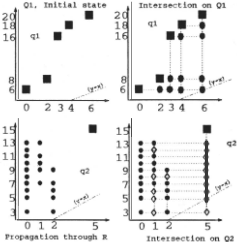
When extending ATMS so as to merge interval semantics (intersection and inclusion rules) and assumption management, some optimization ts obtained.
- Intersection with as..'iumptions: any intersection of n intervals is in fact the intersection of two of them. Computing the intersection of an intersection is unnecessary as it would only give bigger environ ments. Superfluous justifications arc thus removed.
- Inclusion with assumptions: by logical subsumption, bigger intervals that hold under bigger environments can be suppressed, since this redun dancy remains valid through propagation thanks to monotonicity. Thus the only pairs (datum,environment) which arc kept arc those that arc minimal for the following order
( (q, i 1) ,et)::<:;;( (q, i 2) ,e2) ¢> (i 1s;i 2) A (ets;e2). Labels are thus simplified, nodes may be removed and inclusion justifications are not recorded.
Total optimization now leads to the computation of only 18 new data, 28 new justifications and the sup pression of 3 initial data.
2.2.4 Focusing on Nogoods
Previous optimizations arc still insufficient to prevent a combinatorial explosion. We now have to define a propagation procedure which exploits the fact that, for diagnosis purposes, only minimal nogoods are needed . The idea is to propagate only minimal values for each quantity, so as to detect the contradictions (thanks to monotonicity none is missed) . In our example, CATS just computed (q1,[0,6J)n(q1,[6,20))=(q1,[6,6)) and fired ruler ((q1,[6,6)), (q0,[8,9])) --+ (q2,[2,3], which detected a contradiction by intersection with ( q2, [5, 15]) and thus produced the nogood {h1,h2,h3,h4,h5} (see Figure 2).
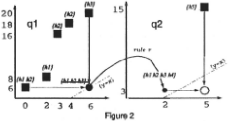
The minimality of the nogoods thus obtained is not guaranteed . CATS therefore uses the recorded path leading to the contradiction to compute minimal values larger than those leading to the contradiction, then activates them. These values may have been com puted previously and in this case were hibernating. In our example, CATS computes (q1,[4,6]) and ( q 1, [6, 6)) using the intersection rule and reactivates (qEl,[7,13]). Ruler is then used with (q0,[8,9)) and the new computed values of q 1 to create ( q2, [2, 5]) and (q2,[0,3)), and with (q1,[6,6)) and the reacti vated value of of q0 to create ( q2, [1, 7]). Intersection is then used first to create (q2,[5,5]) and then (q2,0) under {h1,h3,h4,h5} (see figure 3).
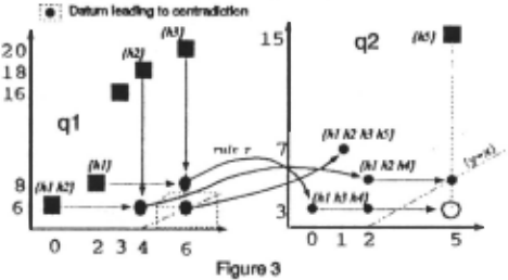
A contradiction thus remains and a smaller nogood {h1,h3,h4,h5} is obtained. The process is repeated: ( q 1, [6, 16]) is computed by intersection and ( q2, [0, 8)) through rule r. As no contradiction is now detected, propagation stops. The final situation is shown in Pigure 4 where [ 4, 6] and [6, 16) are the minimal values for q1 which do not lead to a contra diction. Only 10 new data and 12 new justifications have been created. Sec [Dague ct a!., I 990b] for a detailed description of the algorithm.
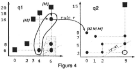
2.3 Extension to Arrays of lnten·als
Up to now, only (quantity,interval) data have been considered. Taking variations of quantities over time into account means here manipulating data that arc arrays of numeric intervals, because of the sampling of quantities. Propagation of arrays raises no particular problems because most computations arc local to a sample, with a few exceptions such as the derivative of a given datum (q,i) that we approximate by (q',i') where i't = (it H e it -6) I 2(5 ( J is the sampling incre ment and e is the difference between intervals) .
Applying the previous techniques of propagation by interval rules, label computation and reactivation of hibernating values to each sample of an array is impracticable (several hundred samples per array). For this reason, we take each array as a whole. The array semantics can now be described by three array rules. The array intersection rule creates the same array as would have been obtained by the intersection rule per element , but only one justification is created. The array falsity rule holds as soon as the falsity rule holds for one element of the array, i.e. if one clement is the empty interval. We arc thus sure to detect all discrep ancies . However, the array inclusion rule between (q,i) and (q,j) applies only if every clement it is included in j 1 . Logical subsumption is not therefore applied when some, but not all , of it arc included in j 1 . Environments computed for the whole array arc in general larger than those that would have been computed for each interval. Consequently, not all minimal conflicts are obtained.
One way to recover the minimal nogoods for a con tradiction is to apply the previous interval algorithm to each sample (that has an empty interval) involved in the contradiction, using the justifications path that leads to it. The correct local label for these samples can thus be computed and hibernating intervals reactivated . As in general these samples arc few in number corn pared to the size of the arrays, this method becomes tractable.
2.4 lmpl<'mcntation
The present implementation (with IDM Prolog and the object-oriented language IPW) of our diagnostic program docs not incorporate aU the features of CATS described here. To simplify programming, we have not yet implemented the complete reactivation procedure or the technique to recover (possibly smaller) conflicts between intervals once a conflict between arrays has been found. Not all minimal conflicts are therefore necessarily obtained. Moreover, although the algo rithm can work on labels made up of more than one environment, our implementation has been limited to just one because two equal intervals are virtually never obtained.
However, our program offers substantial improve ments over the previous one, DIANA [Dague et al ., 1990a]. Firstly, intersections of intervals are processed completely; secondly, there is no limit to the number of times a rule can be fired in a given propagation path; lastly, at the end of propagation, it is now pos sible to reactivate each hibernating value in turn (and not only when the active value becomes inconsistent as was the case in DIANA) .
3 Diagnosing Oscillators
3.1 The Ca.<re of Oscillators
We had already experimented our algorithm on various kinds of circuits but when we tried to diagnose oscillators the results were poor. It so happens that most of the faults which may occur bring the oscillator to a state where all voltages are steady. The reason is that the feedback loop which is at the heart of the circuit cannot accommodate deviations from nominal behavior due to a faulty component, even less so as the feedback for oscillators is positive: correct compo nents are drawn to their limit states, sometimes break down themselves, and all electrical quantities remain con~tant. As a consequence, many components do not appear to be malfunctioning while the diagnostic program i~ applied; it is the case, for instance, for a capacitor if the voltage at the terminals does not vary, or for a transistor which remains saturated (here the collector current is badly defined) . More generally, it is the case when an equation describing a model is not determined for the parameters of the component.
To improve the situation it is necessary to add an external stimulation so as to disturb the circuit and then to perform diagnosis on the disturbance. The fact that a global model of the behavior of the circuit is not required means that there arc few constraints in the choice of stimulation: almost any kind of stimulus can be chosen provided this causes variations in the voltage at the different nodes.
3.2 Advantages of Using External Stimulation
We carried out our experiment on the astable multivi brator shown below.
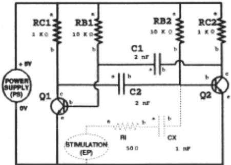
We have studied 12 cases of failure. Taking into account the symmetry of the circuit, they correspond to all the short circuits and aU the breaks in the circuit that could occur in each component. Although the failurcs considered are the most frequent ones, they only represent a small fraction of all possible faults; the results should therefore not be analyzed in statistical tenns. We started by performing diagnosis without stimulation and in this case aU observed voltages were constant. We then applied a pulse which lasted l Jl.S to the base of the transistor q2 via a capacitor ex of 1 nf (dotted lines on the diagram). The results obtained arc summarized in the table below. There was a marked improvement in the diagnosis when external stimu lation was introduced. Without stimulation, no diag noses were proposed in 5 cases of failure, because no contradictions appeared; with stimulation, ·diagnoses were proposed for all of these cases. In 2 other cases of failure the diagnosis is more precise (short circuit of rei and cl) and, in the case of cl under single fault hypothesis, the faulty component can be identified .
The residual ambiguity of the diagnoses should not be blamed on our algorithm or its implementation but, on the contrary, is a consequence of the impossibility of measuring all quantities.
| DEFECT | DIAGNOSES WITHOUT STIMULATION | DIAGNOSES WITH STIMULATION |
| short-circuit on rc I | rc I ,q I ,rb I ,c I, {c2} x {ps,cp,q2,rb2,rc2,ri} | rcl,ql, {c2} x {ps,cx,cl,ep,q2,rbl,rb2,rc2,ri} |
| short-circuit on rb 1 which induces destruction of q 1 | qP | qll |
| short-circuit on c 1 | cl ,ql,rbl | c I, and 10 double candidates |
| short-circuit on q 1 (collector-emitter) | nil | ql,c2, {ret} x {cx,cl,ep,q2,rb2,rc2,ri} |
| short-circuit on q 1 (base-emitter) | ql,cl ,rbl | q I ,c I ,rb 1 |
| short-circuit on q 1 (base-collector) | q I ,cl ,rb 1 ,rei , {c2} x {ps,ep,q2,rb2,rc2,ri} | q 1 ,c I ,rb 1 ,rc 1, {c2} x {ps,cp,q2,rb2,re2,ri} |
| open circuit on rc 1 | nil | rcl,ql,c2 |
| open circuit on rb I | rbl,ql,cl | rbl,ql,cl |
| open circuit on c l | nil | c 1 ,q2,rc2 |
| open circuit on q l (emitter) | ql | ql |
| open circuit on ql (base) | ql | ql |
| open circuit on q 1 (collector) | nil | q I ,c I ,rb I ,c2,rc I |
We know that the use of fault models could help to reduce the ambiguity in our example where the faults tested for came from an existing list of possible faults. Unfortunately such a list can in no way cover all the cases in analog electronics.
4 Conclusion
We have presented an ATMS-like constraint propa gation engine for processing arrays of numeric inter vals, focusing on the recognition of aU minimal nogoods. This engine, CATS, constitutes a powerf~l tool for model-based diagnosis of continuous dynamtc physical systems.
Its application to analog electronics allows the han dling of failures observable only in transient modes and does not require a description of the nominal behavior.
However, as has been shown in this paper, there are cases where, if a system has failed, taking measure ments under the conditions where the failure was detected is not sufficient for model-based diagnosis to be performed. It is necessary to introduce external stimulation and to observe the resulting disturbances in order to obtain a diagnosis. Fortunately, since a global model of the behavior of the circuit is not required for diagnosis, a great scope in the choice of stimulation is possible, as can be seen througl1 the example of oscillators. All we have to do is to kick the ant-hill and see what happens.
Acknowledgments
We would like to thank the referees for their pertinent remarks which enabled us to considerably improve the ftrst draft of this paper. We also thank Rosalind Greenstein for helping us to squeeze a gallon of ideas into a pint pot of acceptable English.
@inproceedings{ijcai1991p163,
  title     = {When Oscillators Stop Oscillating},
  author    = {Dague, Philippe and Jehl, Olivier and Deves, Philippe and Luciani, Pierre and Taillibert, Patrick},
  booktitle = {Proceedings of the Twelfth International Joint Conference on
               Artificial Intelligence, {IJCAI-91}},
  publisher = {International Joint Conferences on Artificial Intelligence},
  editor    = {John Mylopoulos and Ray Reiter},
  pages     = {1109--1114},
  year      = {1991},
  month     = {8},
  note      = {Qualitative Reasoning},
  url       = {https://ijcai.org/proceedings/1991/163},
}
TY - CPAPER TI - When Oscillators Stop Oscillating AU - Dague, Philippe AU - Jehl, Olivier AU - Deves, Philippe AU - Luciani, Pierre AU - Taillibert, Patrick T2 - Proceedings of the Twelfth International Joint Conference on Artificial Intelligence, IJCAI-91 PB - International Joint Conferences on Artificial Intelligence PY - 1991 SP - 1109 EP - 1114 UR - https://ijcai.org/proceedings/1991/163 ER -Copied
Machine-readable versions of this paper, for tools and AI agents:





