"Physical Negation" Integrating Fault Models into the General Diagnostic Engine

1 Introduction

In many systems for model-based diagnosis, the model of the device under consideration captures only the normal, or intended behavior of its components. In exploiting the Assumption-Based Truth-Maintenance System (ATMS), the General Diagnostic Engine (GDE) of [de Kleer-Williams 87) provides an elegant and general framework for this type of diagnostic reasoning. The system assumes the correctness of each component and identifies conjunctions of such correctness assumptions that contradict the observations (measurements). The diagnostic process is then organized as a cycle of gathering more information that helps to decide which correctness assumption(s) should be retracted in order to remove the existing contradictions.

The advantages of GDE, besides being model-based, are that it can handle multiple faults, and it does not require fault models.

On the other hand, GDE does not exploit knowledge about the faulty behavior of components. The

2l SIEMENS Corp. Otto-Hahn-Ring 6 D-8000 Muenchen 83 West Germany dressler@ztivax.siemens.com

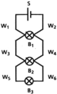
Figure 1

simple example shown in Fig. 1 demonstrates that this can be a drawback: a battery, S, is connected to three bulbs, B1, 82, B3, of the same type. (In order to reduce the number of components involved, we assume that the connections, Wt, ... ,W6, are directly attached to the bulbs.) Suppose we observe that only B3 is lit. Without requiring further measurements, we will come up with the plausible diagnosis {Bt, 82}, meaning that B1 and B2 are broken. This is because the light of B3 indicates the battery supplies sufficient voltage, and a bulb that is not lit despite this fact is considered to be broken (or to have no contact).

What will GDE derive from this situation? It suggests a variety of diagnoses (as we will show in detail in section 2) . Among them is our preferred diagnosis, {Bt , B2}. but also candidates like

{S, 83}, {Wl, Ws}. and others.

The diagnosis {S, 83} explains the observations by a fault in the battery and in the light bulb B3: "The battery does not supply voltage (that is why B1 and B2 are not lit) , and B3 is faulted: it is lit although there is no voltage"! And {W 1, W s} says "B 1 and B 2 are not lit because the wire W1 is broken, and B3 is lit because the wire Ws is behaving improperly: it produces voltage"!

We do not accept these explanations as possible diagnoses because, unlike GDE, we use not only knowledge about the correct behavior of the involved components but also knowledge about their possible behavior when they are faulted. E.g. being lit without voltage supply is not a potential fault of a light bulb.

The example demonstrates that knowledge about the faulty behavior can be very important. In many cases, the diagnostic process involves both

• generating candidates, or diagnostic hypotheses, by identifying sets of components whose correct functioning contradicts the observations, and
• generating explanations, or confirming diagnoses, by analyzing whether the malfunctioning of a (set of) component(s) is consistent with the observations.

GDE carries out the first task, but not the second. The ultimate reason for this lies in what one might call the difference between logical negation and "physical negation": If the retraction of a correctness assumption for a component removes the existing contradictions, this means that the logical negation of the component's correctness is consistent with the observations. It states that the component does not behave according to the normal model, but except for this, it may behave in an arbitrary way.

However, if a component really breaks, i.e. after the "physical negation" of its correctness, it does not operate in a completely unconstrained manner. In many cases, it will still behave in a deterministic, describable way. There may be a number of such modes known, which are called fault models.

Hence, extending GDE in order to capture and exploit fault models appears to be promising. In this paper, we show that this is possible in a very coherent way. Since fault models are applied under the assumption that the respective component is not correct, and since a component is either correct or not, we have to use an extended version of the ATMS that is capable of handling negation and disjunction. Based on this, we are able to make inferences like "If none of the fault models of a component is consistent with the observations then it is correct", or "If each of the fault models of a component is inconsistent with the observations and the correctness of some other component then it is not a candidate for a single fault".

The following section briefly summarizes the structure of GDE and the use of the ATMS in this framework. In section 3, we will state the goal for the integration of fault models and present an extended version of the ATMS. This is shown to establish the required basis for the exploitation offault models: It is possible to infer the correctness of components (section 4), and the use of fault models improves the basis for controlling the diagnostic process (section 5). Perspectives are briefly discussed at the end.

2 GDEandATMS

In this section, we will sketch the basic principles of GDE, using the example introduced above. GDE is supplied with a model of the device in terms of correctly working components. The component models are encoded by constraints which deduce values of system parameters from other known values. This inference process is based on ob$ervations, i.e. input/output data and intermediate measurements. GDE iteratively performs the following steps:

• Prediction: Based on the assumption that each component works correctly, compute values for system parameters.
• Conflict detection: identify those correctness assumptions that are involved in the computation of contradictory values for parameters.
• Candidate generation: construct sets of correctness assumptions that account for the known conflicts (i.e. their conjunctive retraction would remove the contradictions).
• Measurement suggestion: propose measurements that are likely to help discriminating among the candidates.

When new observations are entered, new predictions are made. The process stops when some candidate is an acceptable diagnosis according to some (e.g. probabilistic) criterion.

The measurement suggestion in [de Kleer-Williams 87] is based on probabilistic methods. However, since it is a module quite independent of the others, it could be supplemented or replaced by other knowledge sources and will not be discussed in this paper (Ways for integrating fault models and probabilities are presented in [Hamscher 88) and [de Kleer-Williams 89 )) .

Conflict Detection

If two contradictory values are computed for the same parameter, the correctness assumptions underlying these computations establish a conflict. At least one of these assumptions must be wrong. (In reality, it might be a problem to decide whether or not two values are contradictory as opposed to merely reflecting imprecise measurements, see [Dague-Deves-Raiman 87], [Struss 88a]) .

For describing conflicts, the system has to identify the correctness assumptions a derived value depends on, and, hence, to record the dependencies among the single predictive inference steps. This is done by using the ATMS ([de Kleer 86a]). In the prediction process, each application of a constraint is based on both the parameter values and the assumption that the component works in accordance with its description. This information is transferred to the ATMS.

In principle, the ATMS works as follows : It creates a node for each problem solver datum given to it

(Nodes will be written in capital letters in the following). If the problem solver infers a datum from a conjunction of other data, the ATMS records this dependency as a justification which relates the respective nodes. In our example, we have justifications like

For brevity, each correctness node will be denoted simply by the name of the respective component: e.g. CORRECT(S) = S .

Distinct from the ATMS nodes, there are assumptions (written in small letters), representing the decision of the problem solver to believe or hypothesize that a certain datum is true, e.g. s = correct(S) denotes the assumption of the correctness ofS. The task of the ATMS is to compute the environments for each node, i.e. those sets of assumptions that allow the derivation of this node. Obviously, S has the environment { s}. If a derived node becomes an antecedent for another justification, its environments are combined with those of the other antecedents and propagated to the newly derived node. Thus, via the first justification shown above, VOLTAGE1(S)= + also receives the environment { s }, The node LIGHT(B 1) =ON gets {s, w1, w2 , b1}, because it is justified by Bt's correctness and the necessary voltage drop which in turn depends on the wires, W 1. W 2, and the battery working correctly. The ATMS computes minimal environments (w.r .t . set inclusion) . If a node holds in the empty environment, it is universally true; it is a fact .

There is a distinct node, FALSE, that represents inconsistency. FALSE may have justifications, in our case the existence of conflicting values:

Sets of assumptions that allow to derive FALSE (i.e. inconsistent conjunctions) are called nogoods. Because each superset of a nogood is also in­ consistent, the ATMS computes the set of minimal nogoods as an efficient representation of the existing contradictions. Since we observed that Bt is not lit, i.e. LIGHT(B 1) =OFF is a fact, we obtain

This exemplifies how the ATMS performs the task of conflict detection, and it shows that automatically minimal conflicts are generated. In our example, the following minimal conflicts are identified:

{ S, W1, W2, b1 }, { S, W1 , W2, WJ, W4, b2}, { b3, W5, W6, b2 }, and { b3, WJ, W4 , W5, W6, b1 }.

Candidate Generation

A candidate is a set of components, or rather, their respective correctness assumptions, that accounts for all known conflicts. The underlying idea is that retracting all correctness assumptions of a candidate (which means considering the components as faulty) removes all contradictions with the observations so far. In this sense, a candidate .is a diagnostic hypothesis.

Each candidate has to contain at least one element out of each minimal conflict. For the sake of a compact description of all candidates, again it suffices to construct the candidates that are minimal w.r. t. set inclusion. From the conflicts described above, GDE derives not less than 22 minimal candidates, including the following with 2 elements:

This confirms our claim in the introduction. We see that all but the last one of the 2-element candidates are not acceptable diagnoses, since they contain either a wire that produces voltage out of nothing or a bulb lit without voltage. Only further measure­ ments would enable GDE to rule out implausible diagnostic hypotheses. As we stated in the introduction, the reason for this deficiency lies in the purely logical nature of negating correctness: it allows arbitrary faulty behaviors, excluding only the correct one . Something is missing that is very essential for real diagnostic reasoning: knowledge about what specifically might happen under a fault occurring.

3 Integrating Fault Models

3.1 The Problem

We extend the components' models by descriptions of the behavior they exhibit when they fail. Since different failures may lead to different faulty behaviors, the component models can contain a number of fault views capturing the various fault models of the component. Like the normal models, these fault models are represented by constraints. But they can be activated (and deactivated) independently. A general framework for structured models and their controlled application is described in LStruss 88a, b].

What do we need in order to exploit the fault models?

• If a component, C, has nc distinguishable ways of failing, which are described by fault models, then, if C is generally correct, it is correct w.r.t each of"these fault views:

Vi :S nc CORRECT(C) => CORRECT/C) (This statement assumes that each fault can be detected and not be compensated by others).

• If we want to express that there are no other ways for C to fail, i.e. the fault models are considered complete, we add

CORRECT1(C) 1\ . .. 1\ CORRECTn (C) => CORRECT(C) . c There are no problems in expressing these statements as justifications in the basic ATMS (see Fig. 2 where Ci stands for CORRECT/C) and the dashed circles and arrows indicate the supporting assumptions).

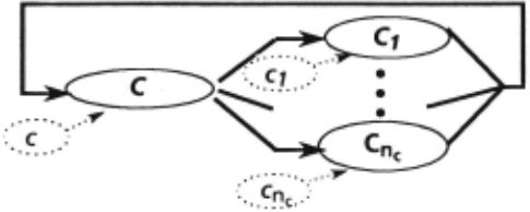
However, when applying fault models, we assume that CORRECT/C) is not true, and we have to express the disjunction that a component is either correct or faulty. Extended versions of the ATMS that allow us to encode negation and disjunctions have been described by [Dressler 87] and [de Kleer 88] . Here, we will briefly summarize the essential features of the extensions required to solve our problem. (For a detailed discussion of their properties in particular in relation to non-monotonic logic, see [Reinfrank et al. 89]).

3.2 An Extended ATMS

The basic ATMS as described in section 2 allows a problem solver to hypothesize or believe the truth of a node, No, by creating an assumption, no, for it (Remember the convention of using capital letters for nodes and small letters for assumptions). The extended ATMS provides a way to explore the consequences of the assumption that No does not hold . This assumption, denoted -.no, supports the corresponding node, -.No.

Two rules in the extended ATMS establish the desired relation between the nodes No and -.No (and their respective assumptions):

• The consistent belief rule states that No and -.No cannot both be true at the same time. It creates justifications such as:

• The nogood inference rule expresses that one of No and -.No must hold. It enables the problem solver to exploit knowledge about inconsistent environments. If E is an environment, and E U {-.no } is inconsistent, then it must be the case that No holds in E. Therefore, for any detected nogood that contains a negated assumption,

this rule creates the justification

In particular, from nogood{ -.no}, No is inferred to hold in the empty environment, i.e. No is established to be a fact .

In [Dressler 88], it is shown that the two rules suffice to achieve the desired effect. -.N0 holds in a consistent context if and only if No does not. Our solution for using fault models in the GDE framework exploits the nogood inference rule extensively, as is shown in the next section.

4 Fault Assumptions - Inferring Correctness of Components

We use the facilities provided by the extended ATMS in the following way: For each fault model of a component, C, two nodes are created, Ci =CORRECT/C) representing "Cis correct w.r.t. the i-th potential fault mode" and -. Ci. Each conclusion drawn from the use of the i-th fault model receives -.ci as a supporting node which is based on the respective fault assumption, 'Ci. As usual, the application of the normal model ofC is supported by the node C, i.e . CORRECT(C), which receives the assumption c.

One motivation for the introduction offault models is to support an inference step like "If each of the known possible failures of a component contradicts the observations, then it is not faulty". We now demonstrate how the extended GDE (Let us call it GDE+> performs this step. The i-th fault model of a component, C, contradicts the observations, if there is a (possibly empty) set of other components, say {A, B }, such that the i-th fault model ofC cannot consistently be joined with any combination of the correct models and fault models of A and B. In terms of assumptions, this means:

Since we have, in particular,

the nogood inference rule of the extended ATMS concludes that all B 1 are valid under all environments { 'Ci, asmA }. Because the conjunction of all B 1 justifies the general correctness of B (consider Fig. 2), these environments are propagated to B. But, since (4.1) also implies that all environments { 'Ci, asmA, b } are nogoods, we get

In the same manner, { -.ci } is detected to be a nogood, and the nogood inference rule derives ci to be a fact. If this is the case for all fault models of C

(i.e. they all contradict the observations) then, based on the completeness of models (Fig. 2), C is established to be true, i.e. C works correctly. The remaining minimal conflicts no longer contain c.

As an illustration, we can now see that GDE + solves the problem of the introductory example. Let each type of component have exactly one fault model, informally stated as:

Battery empty: VOLTAGEt(S)=O

Bulb damaged: LIGHT(B) =OFF

Wire broken:

RESISTANCE(W)=oo

The bulb's only fault model directly contradicts the observation for B3. Hence, B3 is inferred to be correct, and b3 is removed from the minimal conflicts. So a non-zero current at B3 is a fact, which rules out each broken wire and the empty battery. At last, { b1, b2} is the only minimal candidate, as desired. GDE + really got rid of the implausible candidates.

Obviously, this technique for using fault models increases the complexity of GDE and bears the potential danger of creating a huge number of combinations of correct models and fault models some of which may be very unlikely. However, even in such cases, the use of fault models may still be efficient as well as advantageous if combined with appropriate control strategies. This is demonstrated in the following section.

5 Fault Models and Single Fault Assumption

One useful criterion for controlling the diagnostic process is to concentrate on small candidate sets and, in particular, on single faults . Fault models may support such a control regime considerably. For instance, if each fault model of a component, C, under the given observations contradicts the correctness assumption of at least one other component, then the faultiness of C alone cannot explain the observations and, hence, C is not a candidate for a single fault . Without affecting the capability to handle multiple faults, GDE + automatically performs this kind of inferences as the following informally presented example illustrates.

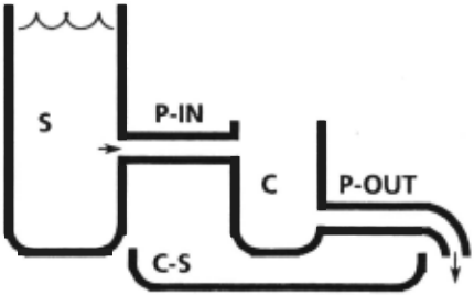
Water is supposed to flow from an infinite water supply, S, through a pipe, P-IN, into a container, C, and from there through pipe P-OUT to the outlet. For security reasons, there is another container, C-S, for capturing water from an overflow or broken pipes (Fig. 3).

Assume, S really contains enough water, and the only available information is

OUTPUT(P-OUT) = O WATER-LEVEL(C-S) = 0.

The correct models of OUTPUT(P-OUT) = +, observation, P-IN, C, P-OUT and, from the imply first

(5.1) {p-in, c, p-out}

is established as the only minimal conflict, which merely indicates that something is wrong on the way from the water supply to the outlet. Generating three minimal candidates, {p-in}, { c }, {p-out}, is all the basic GDE can do. We use GDE+ and supply it with the following fault models (giving their respective fault assumptions reasonable names):

• containers may have holes: hole(C) = -,correct(C)
• pipes may be perforated or clogged: perforated(?) = -,correct1(P) clogged(P) = -,correct2(P) .

If these fault models are activated, the following nogoods will be detected:

(5 .2) {hole(C), p-in, c-s }

(i.e. water running out of C through a hole would be detected in a correct C-S in contrast to the second observation). Similarly, the following no goods are found:

(5.3) {perforated(P-IN), c-s} ,

(5.4) {perforated(P-OUT),p-in, c, c-s } , and, finally,

(5.5) {clogged(P-OUT), p-in, c , c-s }

(If P-IN works, C is also correct, and P-OUT is clogged, then C-S would contain water from the resulting overflow of C). Note that (5.2) through (5.5) are not conflicts, because they include fault assumptions.

From (5 .2), the nogood inference rule creates

This has two results: due to (5.1), a second conflict, (5.6) {p-in, c-s, p-out } ,

is detected, and the nogoods (5.4) and (5 .5) are minimized to

(5.4') {perforated(P-OUT), p-in, c-s } and

(5.5') {clogged(P-OUT), p -in, c-s } .

The nogood inference rule applied to (5.4') and (5 .5') establishes

and, via completeness of P-OUT's fault models, reduces the conflict (5.6) to (5.6') { p-in, c-s } .

The minimal candidates derived from the minimal conflicts, (5.1) and (5.6'), are

and P-IN is the only candidate for a single fault. Moreover, under the single fault assumption, we have information about what is wrong with P-IN: (5.3) excludes PERFORATED(P-IN) from being a single fault and, hence, implies that CLOGGED(P­ IN) is the only possible failure of P-IN.

In this case, the system could not prove the correctness of a component. However, in using fault models, it changed the set of the minimal candidates and provided important information for control decisions, e.g. focusing on P-IN. The core of the performed inferences is the following: If each fault model of C is inconsistent with some set of correct models of other components,

(remember 'Ci = ·correct/C) ) then the nogood inference rule creates justifications

and, via completeness .of fault models, C =CORRECT(C) receives an environment consisting only of correctness assumptions:

This expresses the fact that, regardless of how C fails, this can only be true if some other component is also faulty.

Note that for establishing (5.7), it suffices to consider only combinations of models that contain exactly one fault model. This means the results are derivable without the potential combinatorial explosion that might occur in the correctness proof presented in the previous section. The analysis can be focused on contexts that contain not more than one fault assumption. [Dressler-Farquhar 89] presents a control mechanism based on consumers ([de Kleer 86b]) which is able to perform this task.

6 Perspectives

The completeness of fault models is an essential condition for the inference mechanism presented here. If a faulty component exhibits a behavior that is not captured by one of the fault views, wrong conclusions may be drawn. A reasonable diagnostic strategy is to first assume that only typical or known faults occur, until there is evidence to the contrary. This requires making the assumption about the completeness of fault models explicit . An additional antecedent for the correctness of a component 1s introduced:

CORRECTz(C) I\ ... I\ CORRECTn (C) I\ ELSE-CORRECT(C) ~ CORRECT(C) .

It represents the remaining faults and is supported by an assumption. [Struss 88b, 89], describe how GDE + can reason about such assumptions underlying the diagnostic process (the correctness of observations and the single fault hypothesis are other examples). Again, this is possible without leaving the basic concepts and mechanisms ofGDE.

Acknowledgements

We benefited from discussions with Daniel Bobrow Johan de Kleer, Keith Downing, Hartmut Freitag: Olivier Raiman, and Michael Reinfrank. Thanks to Linda Pfeffer! for her technical support. This work was partly supported by the Bundesminister fuer Forschung und Technologie (ITW 8506 E4).