
Structured Plans and Observation Reduction for Plans with Contexts
Proceedings of the Twenty-First International Joint Conference on Artificial Intelligence. Pages 1721-1726.
© 2009 International Joint Conferences on Artificial Intelligence
Abstract
In many real world planning domains, some observation information is optional and useless to the execution of a plan; on the other hand, information acquisition may require some kind of cost. The problem of observation reduction for strong plans has been addressed in the literature. However, observation reduction for plans with contexts (which are more general and useful than strong plans in robotics) is still a open problem. In this paper, we present an attempt to solve the problem. Our first contribution is the definition of structured plans, which can encode sequential, conditional and iterative behaviors, and is expressive enough for dealing with incomplete observation information and internal states of the agent. A second contribution is an observation reduction algorithm for plans with contexts, which can transform a plan with contexts into a structured plan that only branches on necessary observation information.Wei Huang, Zhonghua Wen, Yunfei Jiang, Hong Peng
- [Bertoli and Pistore, 2004] Piergiorgio Bertoli and Marco Pi- store. Planning with extended goals and partial observabil- ity. In Proceedings of the 14th International Conference on Automated Planning and Scheduling, pages 270-278, 2004.
- [Bertoli et al., 2001] Piergiorgio Bertoli, Alessandro Cimatti, Marco Roveri, and Paolo Traverso. Planning in nondeterministic domains under partial observability via symbolic model checking. In Proceedings of the 17th International Joint Conference on Artificial Intelligence, pages 473-478, 2001. IJCAI
- [Bertoli et al., 2003] Piergiorgio Bertoli, Alessandro Cimatti, Marco Pistore, and Paolo Traverso. A framework for planning with extended goals under partial observabil- ity. In Proceedings of the 13th International Conference on Automated Planning and Scheduling, pages 215-225, 2003.
- [Bertoli et al., 2006] Piergiorgio Bertoli, Alessandro Cimatti, Marco Roveri, and Paolo Traverso. Strong plan- ning under partial observability. Artificial Intelligence, 170:337-384, 2006.
- [Bonet and Geffner, 2000] Blai Bonet and Hector Geffner. Planning with incomplete information as heuristic search in belief space. In Proceedings of the 5th International Conference on AI Planning Systems, pages 52-61, 2000.
- [Cimatti et al., 2003] Alessandro Cimatti, Marco Pistore, Marco Roveri, and Paolo Traverso. Weak, strong, and strong cyclic planning via symbolic model checking. Arti- ficial Intelligence, 147:35-84, 2003.
- [Huang et al., 2007] Wei Huang, Zhonghua Wen, Yunfei Jiang, and Lihua Wu. Observation reduction for strong plans. In Proceedings of the 20th International Joint Con- ference on Artificial Intelligence, pages 1930-1935, 2007. IJCAI
- [Kaelbling et al., 1998] Leslie Pack Kaelbling, Michael L. Littman, and Anthony R. Cassandra. Planning and act- ing in partially observable stochastic domains. Artificial Intelligence Research, 101(1-2):99-134, 1998.
- [Lago et al., 2002] Ugo Dal Lago, Marco Pistore, and Paolo Traverso. Planning with a language for extended goals. In Proceedings of the 18th National Conference on Artificial Intelligence, pages 447-454, 2002.
- [Pistore and Traverso, 2001] Marco Pistore and Paolo Traverso. Planning as model checking for extended goals in non-deterministic domains. In Proceedings of the 17th International Joint Conference on Artificial Intelligence, pages 479-484, 2001.
- [Sardina et al., 2006] Sebastian Sardina, Giuseppe De Gia- como, Yves Lesperance, and Hector J. Levesque. On the limits of planning over belief states under strict uncer- tainty. In Proceedings of the 10th International Confer- ence on Principles of Knowledge Representation and Rea- soning, pages 463-471, 2006.
References were extracted automatically from the PDF and may contain errors.
Full text extracted automatically from the PDF; figures, tables and equations may differ. The PDF is the version of record.
1 Introduction
Planning for extended goals in nondeterministic domains [Pistore and Traverso, 2001; Lago et al., 2002], is a well known and significant problem in AI. In nondeterministic and full observable domains, actions are modelled with different outcomes that cannot be predicted at planning time, and the state of the world can be completely identified via some possible observation at execution time. Therefore, it is the job of plans to specify what to do depending on the observation information gathered at execution time, and the context of execution, i.e., the internal state of the agent.
The plan synthesis problem has been addressed in the literature (e.g., see [Pistore and Traverso, 2001; Lago et al., 2002]), where plans are expressed as policies on state-context pairs (i.e., plans with contexts). The agent executing plans with contexts, is considered able to sense the state of the world directly, and depending on the state of the world and the internal state of the agent, execute different actions. In most real world domains, however, the agent distinguishes states of the world by acquiring some optional observation information at some cost (battery, money, and time, etc.). On the other hand, some observation information may be unnecessary to the plan execution. So it is significant to reduce the unnecessary observation tasks for plans with contexts. A simpler subset of this problem, i.e., observation reduction for strong plans [Cimatti et al., 2003] has been already addressed in [Huang et al., 2007], but to the best of our knowledge, observation reduction for general plans with contexts is still an open problem. In this paper, we present a first attempt to solve the problem.
At first, we extend conditional plans [Huang et al., 2007; Bertoli et al., 2006] to structured plans that can encode sequential, conditional and iterative behaviors, and are expressive enough for dealing with incomplete observation information and with internal states of the agent. Intuitively, structured plans are similar to programs with conditional statements and loops, in which contexts are used to represent the destination points of jumps occurring in execution control. We also define what does "a structured plan is equivalent to a plan with contexts" mean, and the expected cost of observation information acquisition required at every step of the execution of a structured plan.
And then, we define an observation reduction algorithm for general plans with contexts. The algorithm can transform a plan with contexts into a structured plan that only branches on necessary observation information. The algorithm terminates, and is correct (i.e., the structured plan returned by the algorithm is equivalent to the plan with contexts).
This paper is structured as follows. Firstly, we review some basic notions that are relevant to our work (see [Pistore and Traverso, 2001; Huang et al., 2007] for further details and examples). Secondly, we introduce some definitions about structured plans and their execution. Thirdly, we describe an observation reduction algorithm for plans with contexts, and show some properties of the algorithm. Finally, we draw some conclusions and discuss future research directions.
2 Preliminaries
A planning domain Σ = 〈S, A, I, R〉 is a model of a generic system with its own dynamics, where S is a finite set of states, A is a finite set of actions, I ⊆ S is the set of initial states (we require I ̸= ∅), and R : S ×A → 2S is the state-transition function. ACT(s) = {a ∈ A|∃s′ ∈ R(s, a)} denotes the set of actions that are applicable in s ∈ S.
A plan with contexts πC for Σ is a tuple 〈C, c0, act, ctxt〉 where: C is a set of contexts, c0 ∈ C is the initial context, act : S × C → A is the action function, and ctxt : S × C × S → C is the context function. The execution of πC on Σ can be described in terms of transitions between statecontext pairs: 〈s, c〉-→a 〈s′ , c′ 〉 if s′ ∈ R(s, a), a = act(s, c), and c′ = ctxt(s, c, s′ ). A run of plan πC from state s0 is a possibly infinite sequence 〈s0, c0〉-→a0〈s1, c1〉-→a1 . . . where 〈si, ci〉-→ai 〈si+1, ci+1〉 are transitions. The execution structure K = 〈SC, SC0, T R〉 is the finite presentation of the set of all possible runs of πC on Σ, where:
- SC0 = I ×{c0};
- SC is the minimal set satisfying the following rules:
- if 〈s, c〉 ∈ SC, and there exists a ∈ A and 〈s′ , c′ 〉 ∈ S × C such that 〈s, c〉-→a 〈s′ , c′ 〉, then 〈s′ , c′ 〉 ∈ SC;
- and 〈〈s, c〉, 〈s′ , c′ 〉〉 ∈ T R if 〈s, c〉-→a 〈s′ , c′ 〉 for some a.
The agent executing plans with contexts, is considered able to sense the state of the world directly, and depending on the state of the world and the internal state of the agent (i.e., the context), execute different actions. In practice, however, the agent distinguishes states of the world by acquiring some optional observation information at some cost (e.g., time, money, and power etc.). An observation setting can be modelled by a set of observation variables V, and an observation function X : S ×V → {⊤,⊥}. 1 The observation of a set of states ∅ ⊂ S ′ ⊆ S built on ∅ ⊂ V ′ ⊆ V and X can be expressed as a propositional formula, and it is:
O(S, V, X) = {OBS(S ′ , V ′ , X) | ∅ ⊂ S ′ ⊆ S, ∅ ⊂ V ′ ⊆ V} is the set of all possible observations built from 〈S, V,X〉. Furthermore, for each observation variable v ∈ V, we use an integer COST(v) to represent the cost of each time sensing the value of v.
In the following example 2 , that will be used throughout the paper, we will illustrate the notions introduced in this section.
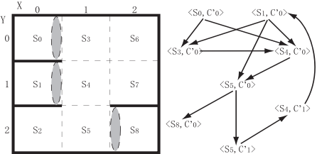
Example 1 The left of Figure 1 shows a simple robot navigation domain Σ which contains a 3 × 3 room. The states of Σ (i.e., S = {s0, . . . , s8}) correspond to the 9 positions in the room. s0 and s1 are the possible initial states of Σ, i.e., I = {s0, s1}. The robot can move in the four directions (i.e., A = {→, ↓,←, ↑}). An action is applicable only if there is no wall in the direction of motion. All the actions are deterministic (e.g., R(s3, ↓) = {s4}), except for action → :
1 In fact, 〈V, X〉 can be used to model partial observability (e.g., [Bertoli et al., 2001; 2006]). However, for the sake of executability of plans with contexts, we assume that any two distinct states of the world can be distinguished by one observation variable at least.
2 The planning domain and the observation setting introduced in this example are modified from those given in [Huang et al., 2007].
| s | c | act(s, c) | s′ ∈ R(s, a) | ctxt(s, c, s′ ) |
| s0 | c′0 | → | s3 or s4 | c′0 |
| s1 | c′0 | → | s3, s4, or s5 | c′0 |
| s3 | c′0 | ↓ | s4 | c′0 |
| s4 | c′0 | ↓ | s5 | c′0 |
| s5 | c′0 | → | s8 | c′0 |
| s5 | c′0 | → | s5 | c′1 |
| s5 | c′1 | ↑ | s4 | c′1 |
| s4 | c′1 | ← | s1 | c′0 |
- when on s0 (or s1), the robot may slip and end up either in s3 or s4 (or in s3, s4, or s5), i.e., R(s0,→) = {s3, s4} and R(s1, →) = {s3, s4, s5};
- when on s5, the robot may be blocked by a door and end up either in s5 or s8, i.e., R(s5,→) = {s5, s8}.
Let πC = 〈C ′ , c′0, act, ctxt〉 be the plan with contexts shown in Table 1. The execution structure K corresponding to πC and Σ is shown on the right of Figure 1.
Suppose the robot can detect the position of the walls neighboring its location, and perceive whether the Xcoordinate (or Y-coordinate) of its location is n(0 ≤ n ≤ 2) (i.e., the set of observation variables V = {E,S,W,N,X0,X1,X2,Y0,Y1,Y2}). So the observation function X is such that X(s0, E) = ⊥, X(s5, X1) = ⊤, and so on. OBS(I, {E,S}, X) = ¬E ∧ S. For the sake of simplicity, we assume that COST(v) = 1 for each v ∈ V. The agent executing πC, has to observe all the observation variables before it selects an action to execute. Hence, the total cost of observation information acquisition required at every step of the execution of πC is ∑v∈V COST(v) = |V| = 10.
In the rest of this paper, Σ = 〈S, A, I, R〉, V, and X represent a planning domain, a finite set of observation variables, and an observation function over S and V, respectively.
3 Structured Plans
In this section, we present the definition of structured plans, which can encode sequential, conditional and iterative behaviors, and is expressive enough for dealing with incomplete observation information and with internal states of the agent.
Intuitively, structured plans are similar to programs with conditional statements and loops. An empty plan ε means doing nothing except sending a signal of termination. Contexts work as destination points of jumps that take place in execution control, and the initial context represents the place where the whole execution begins. For each context, the explanation function specifies the rest of the plan to be executed from the point corresponding to the context.
Definition 1 A structured plan for 〈Σ, V, X〉 is a tuple πS = 〈C, c0, E〉, where C is a finite set of contexts, c0 ∈ C is the initial context, and E : C → Π is the explanation function. Π is the set of sub-plans built on 〈Σ, V,X, C〉, and it is the minimal set satisfying the following rules:
- C ∪ {ε} ⊆ Π, ε is the empty plan;
- if a ∈ A and π ∈ Π, then a ◦ π ∈ Π;
- if ∅ ⊂ V ′ ⊆ V, and 〈oi, πi〉 ∈ O(S, V ′ ,X) ×Π for all 1 ≤ i ≤ n, then switch(V ′ ){〈oi, πi〉|1 ≤ i ≤ n} ∈ Π.
In the following discussion, πS = 〈C, c0, E〉 represents a structured plan for 〈Σ, V,X〉. We say that πS is simple, if C ∩ {E(c)|c ∈ C} = ∅. Intuitively, successive jumps are not allowed in the execution control of a simple structured plan. In the rest of the paper, we consider only structured plans that are simple. If o, o′ ∈ O(S, V,X) and o → o′ is a tautology, then we write o ⇒ o′ .
The execution of πS is defined in terms of the runs associated to it. Intuitively, a run σ is a sequence of configurations [Sardina et al., 2006] that, describe the world state, the belief state [Bonet and Geffner, 2000], and the rest of the plan to be executed.
Definition 2 A configuration for 〈Σ, V,X〉 and structured plan πS is a tuple 〈s, B, π〉 ∈ S × 2S × Π.
Configuration 〈s, I, E(c0)〉 is initial if s ∈ I. Configuration 〈s, B, π〉 may evolve into configuration 〈s′ , B′ , π′ 〉, written 〈s, B, π〉 -→ 〈s′ , B′ , π′ 〉, if either:
- π = a ◦ π′′ , if π′′ ̸∈ C then π′ = π′′ else π′ = E(π′′ ), s′ ∈ R(s, a) and B′ = ∪s′′ ∈BR(s′′ , a); or
- π = switch(V ′ ){〈o1, π1〉, . . . , 〈on, πn〉}, OBS({s}, V ′ ,X) ⇒ oi, if πi ̸∈ C then π′ = πi else π′ = E(πi), s′ = s, and B′ = {s′′ ∈ B|OBS({s′′}, V ′ , X ) ⇒ oi}.
The reachable configurations for 〈Σ, V, X 〉 and πS , are defined by the following rules:
- if 〈s, B, π〉 is initial, then it is reachable;
- if 〈s, B, π〉 is reachable and 〈s, B, π〉 -→ 〈s′ , B′ , π′ 〉, then 〈s′ , B′ , π′ 〉 is also reachable.
Due to the nondeterminism in a planning domain, there may be many different runs of a structured plan. We use an execution structure to represent the set of all possible runs.
Definition 3 The execution structure corresponding to 〈Σ, V,X〉 and structured plan πS, is K = 〈Q,Q0, T 〉, where: Q is the set of reachable configurations; Q0 = {〈s, I, E(c0)〉|s ∈ I} is the set of initial configurations; and T = {〈q, q′ 〉 ∈ Q×Q|q -→ q′}.
In the following discussion, K = 〈Q,Q0, T 〉 represents the execution structure corresponding to 〈Σ, V,X〉 and πS.
TERC(K) = {q ∈ Q|∀q′ ∈ Q.〈q, q′ 〉 ̸∈ T } denotes the set of terminal configurations of execution structure K. A run of K from q0 is a possibly infinite sequence (q0, q1, . . .) such that, for every qi, either qi ∈ TERC(K) or 〈qi, qi+1〉 ∈ T . RUNS(q,K) denotes the set of runs of K from q.
In general, we are interested in executable structured plans, i.e., structured plans whose execution guarantees that an action is never attempted unless it is applicable, and that for any possible observation information, they say what to do next without ambiguity.
Definition 4 Let K = 〈Q, Q0, T 〉 be the execution structure corresponding to 〈Σ, V,X〉 and structured plan πS. πS is executable on 〈Σ, V, X〉 if:
- for all 〈s, B, π〉 ∈ TERC(K), π is ε; and
- for all 〈s, B, π〉 ∈ Q such that π takes the form of switch(V ′ ){〈oi, πi〉|1 ≤ i ≤ n}, there exists only one 1 ≤ i ≤ n such that OBS({s}, V ′ , X ) ⇒ oi.
Sometimes we may only be interested in the state transitions induced by (the execution of) a structured plan. Let q0 = 〈s0, B0, π0〉 ∈ Q, and σ = (〈s0, B0, π0〉, 〈s1, B1, π1〉, . . . , 〈si, Bi, πi〉, . . .) ∈ RUNS(q0,K), then we use STRS(σ) = s′0 ⋄ a1 ⋄ s′1 ⋄ . . . (where s′i ∈ S, ai+1 ∈ A) to represent the state transitions corresponding to σ such that:
- if π0 = ε, then STRS(σ) = s0; or else
- if π0 = a ◦ . . . such that a ∈ A, then STRS(σ) = s0 ⋄ a ⋄ s′1 ⋄ . . . such that s′1 ⋄ . . . = STRS((〈s1, B1, π1〉, . . . , 〈si, Bi, πi〉, . . .)); or else
- STRS(σ) = STRS((〈s1, B1, π1〉, . . . , 〈si, Bi, πi〉, . . .)).
Now we can compare the behaviors induced by (the execution of) a structured plan πS with those induced by a plan with contexts πC.
Definition 5 Let πC = 〈C ′ , c′0 , act, ctxt〉 be a plan with contexts for Σ. Then πS is equivalent to πC on 〈Σ, V, X〉 iff:
- for each s0 ∈ I and σ ∈ RUNS(〈s0, I, E(c0)〉,K) such that STRS(σ) = s0 ⋄ a1 ⋄ s1 ⋄ a2 ⋄ . . ., there exists a run σ′ = 〈s0, c′0 〉-→a1〈s1, c′1 〉-→a2 . . . of πC such that c′i ∈ C ′ ;
- and for each s0 ∈ I and run σ′ of πC from s0 (let σ′ = 〈s0, c′0 〉-→a1〈s1, c′1 〉-→a2 . . .), there exists σ ∈ RUNS(〈s0, I, E(c0)〉, K) such that STRS(σ) = s0 ⋄a1 ⋄ s1 ⋄ a2 ⋄ . . .
Definition 5 only concerns the state transitions induced by a structured plan and a plan with contexts. However, in many real world domains, the cost of observation information acquisition is an issue.
Definition 6 Let 〈s0, B0, π0〉 ∈ Q and σ ∈ RUNS(〈s0, B0, π0〉,K) such that σ = (〈s0, B0, π0〉, 〈s1, B1, π1〉, . . . , 〈si, Bi, πi〉, . . .). Then the expected cost of observation information acquisition required at every step of the execution (i.e., choosing an action) corresponding to σ is:
In the following example, we illustrate the definitions given in this section.
Example 2 Consider the situation depicted in Example 1. Let πS = 〈C, c0, E〉 be a structured plan for 〈Σ, V, X〉, where:
- C = {c0, c1}, E(c0) =→ ◦c1,
- E(c1) =switch({S}){〈S,→ ◦π0〉, 〈¬S, ↓ ◦π1〉},
- π0 =switch({E}){〈E, ε〉, 〈¬E, ↑ ◦ ← ◦c0〉}, and
- π1 =switch({S}){〈S,→ ◦π0〉, 〈¬S, ↓ ◦ → ◦π0〉}.
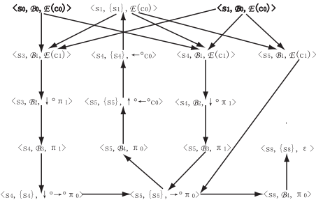
Let B0 = I, B1 = {s3, s4, s5}, B2 = {s3, s4}, B3 = {s4, s5}, and B4 = {s5, s8}. The execution structure K = 〈Q,Q0, T 〉 corresponding to 〈Σ, V, X〉 and πS is shown (as a directed graph) in Figure 2. It is easy to find that πS is simple and executable on 〈Σ, V, X 〉.
In Figure 2, we can find that σ1 = (〈s1, B0, E(c0)〉, 〈s5, B1, E(c1)〉, 〈s5, {s5}, → ◦π0〉, 〈s5, B4, π0〉, 〈s5, {s5}, ↑ ◦ ← ◦c0〉, 〈s4, {s4},← ◦c0〉, 〈s1, {s1}, E(c0)〉, 〈s5, B1, E(c1)〉, . . .) and σ2 = (〈s1, B0, E(c0)〉, 〈s5, B1, E(c1)〉, 〈s5, {s5},→ ◦π0〉, 〈s8, B4, π0〉, 〈s8, {s8}, ε〉) are two runs of K from 〈s1, B0, E(c0)〉. According to definition 6 and the assumption that (∀v ∈ V)COST(v) = 1, AVOC(σ1) = limn→∞2n/(1 + 1 + 4n) = 0.5 and AVOC(σ2) = 2/(1 + 2) ≈ 0.67. Furthermore, πS is equivalent to πC on 〈Σ, V,X〉. For each s ∈ I and σ′ ∈ RUNS(〈s, I, E(c0)〉,K), AVOC(σ′ ) < 1 < |V| (i.e., the cost of observation information acquisition required at every step of the execution of πC).
4 Observation Reduction for Plans with Contexts
In this section, we will introduce an algorithm to observation reduction for general plans with contexts. The algorithm (i.e., OBSREDUCE) is reported in Figure 3. Given a planning domain Σ = 〈S, A, I, R〉, an observation setting 〈V, X〉 on Σ, and a plan with contexts πC = 〈C ′ , c′0, act, ctxt〉 for Σ, it transforms πC into a structured plan πS = 〈C, c0, E〉, which
- procedure OBSREDUCE(πC)
- SCA := SCV := loops := ∅, C = ∅;
- dis := SIMULATE(I × {c′0}, πC);
- Vobs := REDUCE(dis, V);
- for all SC ∈ loops ∪ {I × {c′0}}
- create a context cSC;
- C := C ∪ {cSC};
- for all cSC ∈ C
- E[cSC] := CONPLAN(SC, πC, Vobs);
- return 〈C, cI×{c′0}, E〉;
- end
Figure 3: OBSREDUCE algorithm
is equivalent to πC on 〈Σ, V, X 〉 and only branches on necessary observation information. We assume that 〈Σ, V, X〉 is a global variable.
At every step (i.e., choosing an action) of the execution of πC, the agent only needs to distinguish the current statecontext pair 〈s, c〉 from 〈s′ , c′ 〉 ∈ SC (SC is the set of possible current state-context pairs) such that:
- the action specified by πC on 〈s′ , c′ 〉 is different from that on 〈s, c〉 (i.e., act(s′ , c′ ) ̸= act(s, c)); or
- the contexts corresponding to some state s′′ will not be identical at next step (i.e., 〈s, c〉-→a 〈s′′ , c1〉 and 〈s′ , c′ 〉-→a 〈s′′ , c2〉 for some a ∈ A where c1 ̸= c2). 3
We can use two state-context pairs (e.g., 〈〈s, c〉, 〈s′ , c′ 〉〉) to represent a basic distinguishing task. In the algorithm, all the basic distinguishing tasks that may arise during the execution of πC from I × {c′0}, are recorded in dis. On the other hand, πC may result in iterative behaviors. Therefore, during the execution of πC, some loops of sets of state-context pairs encountered may arise. In the algorithm, all the entrances of these loops, and all the sets of state-context pairs encountered, are recorded in loops and SCV respectively. SCA records the sets of state-context pairs encountered in some runs of πC (i.e., SCA is the current set of state-context pairs). loops, SCV , and SCA are all global variables.
Initially, the recursive procedure SIMULATE(I×{c′0}, πC) is called to calculate dis (line 3). And then, REDUCE(dis, V) is called to calculate Vobs ⊆ V such that (∀〈〈s, c〉, 〈s′ , c′ 〉〉 ∈ dis)(∃v ∈ Vobs)X(s, v) ̸= X(s′ , v) (line 4). So at every step of the execution of πC from I × {c′0}, the agent does not need to consider the values of the observation variables in V - Vobs. At last, for each SC ∈ loops ∪ {I × {c′0}}, the algorithm creates a distinct context cSC to represent the place where E[cSC] (i.e., the rest of the plan πS to be executed form SC) begins (lines 5-7), and calls the recursive procedure CONPLAN(SC, πC, Vobs) to construct E[cSC] that only branches on some subset of Vobs (lines 8-9). The initial context that represents the place where the whole execution begins, is set as cI×{c′0} (line 10).
3 For example, consider the situation and plan πC depicted in Example 1. Initially, it makes no sense to observe the value of any v ∈ V because (∀s ∈ I)(act(s, c′0) =→) ∧ (∀s′ ∈ R(s,→ ))ctxt(s, c′0, s′ ) = c′0. If we modify πC such that ctxt(s0, c′0, s4) = c′1, then s0 should be distinguished from s1 because different actions (i.e., ↓ and ←) will be executed on s4 at next step.
SIMULATE, REDUCE, and CONPLAN subroutines are shown in Figure 4 and Figure 5. Now let us introduce them.
SIMULATE(SC, πC) calculates the set of basic distinguishing tasks dis ⊆ (S × C ′ )2 that may arise during the execution of πC from SC. Its basic idea is to simulate the behaviors induced by πC from SC. During the simulation, the entrances of loops (i.e., loops of sets of state-context pairs encountered) are recorded in loops (lines 13-14); and according to the actions specified by πC and the successive state-context pairs, the possible current state-context pairs are dealt with separately (lines 18-24, and lines 28-38 4 ).
Given dis ⊆ (S × C ′)2 and ∅ ⊂ V ′ ⊆ V as input, the procedure REDUCE returns Vobs ⊆ V ′ such that (∀〈〈s, c〉, 〈s′ , c′ 〉〉 ∈ dis)(∃v ∈ Vobs)X(s, v) ̸= X(s′ , v). It starts with Vobs = ∅ and iteratively adds some v ∈ V ′ (whose observation cost per basic distinguishing task is minimal, see line 71) into Vobs until d = dis, where d = {〈〈s, c〉, 〈s′ , c′ 〉〉 ∈ dis |(∃v ∈ Vobs)X(s, v) ̸= X(s′ , v)}.
For the execution of πC started from SC ⊆ S ×C ′ , CONPLAN(SC, πC, Vobs) constructs the corresponding part of πS, which only branches on some subset of Vobs. VPLAN is similar to CONPLAN except that it checks whether SC is an entrance of a loop (line 61). In this case, the context corresponding to SC (i.e., cSC) is returned by VPLAN. The basic idea of CONPLAN is similar to that of SIMULATE, i.e., it is to simulate the behaviors induced by πC from SC. If two possible current state-context pairs in SC should be distinguished from each other, then the executions of πC started from them, will be simulated separately (line 41, and lines 44-58).
We now show some properties of the algorithm OBSREDUCE(πC). To do so, we first introduce the notion of SCS(I×{c′0}, πC). SCS(I×{c′0}, πC) is the minimal set satisfying the following rules:
- I × {c′0} ∈ SCS(I × {c′0}, πC);
- if SC ∈ SCS(I × {c′0}, πC), and DIVIDE(SC, πC) = {〈a, SC〉} for some a ∈ A, then EXECUTE(SC, a, πC) ∈ SCS(I × {c′0}, πC);
- if SC ∈ SCS(I × {c′0}, πC), then (∀〈a, SC ′ 〉 ∈ DIVIDE(SC, πC))SC ′ ∈ SCS(I × {c′0}, πC).
In the execution of OBSREDUCE(πC), SCS(I ×{c′0}, πC) is recorded as SCV , which is updated by the calls of SIMULATE (line 17, Figure 4).
Theorem 1 Let K = 〈SC, SC0, T R〉 be the execution structure of a plan with contexts πC on Σ. OBSREDUCE(πC) is guaranteed to terminate, and it is polynomial in |V|, |SCS(I × {c′0}, πC)|, and |SC|.
Proof: See appendix. ■
Theorem 2 When OBSREDUCE(πC) returns a structured plan πS = 〈C, c0, E〉 (let K be the execution struc-
4 Formally, let 〈a, SC ′〉 ∈ DIVIDE(SC, πC) and 〈s, c〉 ∈ SC ′ then (∀〈s′ , c′ 〉 ∈ SC)(〈s′ , c′ 〉 ∈ SC ′) ↔ (act(s′ , c′ ) = a) ∧ (∀s′′ ∈ R(s, a) ∩ R(s′ , a))(ctxt(s, c, s′′ ) = ctxt(s′ , c′ , s′′ )). VAILD(SC, πC) = {〈s, c〉 ∈ SC|act(s, c) is defined in πC}. And EXECUTE(SC, a, πC) = {〈s, c〉|(∃〈s′ , c′ 〉 ∈ SC)〈s′ , c′ 〉-→a 〈s, c〉}.
- procedure SIMULATE(SC, πC) 13. if SC ∈ SCA then 14. loops := loops ∪ {SC}, return ∅; 15. if SC ∈ SCV or VAILD(SC, πC) = ∅ 16. then return ∅; 17. SCA := SCA ∪ {SC}, SCV := SCV ∪ {SC}; 18. divitions := DIVIDE(SC, πC); 19. if divitions = {〈a, SC〉} for some a ∈ A then 20. return SIMULATE(EXECUTE(SC, a, πC), πC); 21. dis = ∅, SC ′ := SC; 22. for all 〈a′ , SC ′′ 〉 ∈ divitions 23. SC ′ := SC ′ - SC ′′ ; 24. dis := dis ∪ (SC ′′ × SC ′ ) ∪ SIMULATE(SC ′′ , πC) 25. SCA := SCA -{SC}; 26. return dis; 27. end 28. procedure DIVIDE(SC, πC) 29. divisions := ∅, SC ′ := VALID(SC, πC); 30. while SC ′ ̸= ∅ do 31. select a pair 〈s, c〉 fromSC ′ randomly; 32. divition := {〈s, c〉}, SC ′ := SC ′ - {〈s, c〉}; 33. for all 〈s′ , c′ 〉 ∈ SC ′ such that act(s′ , c′ ) = act(s, c) and ∀s′′ ∈ R(s, act(s, c)) ∩ R(s′ , act(s′ , c′ )). ctxt(s, c, s′′ ) = ctxt(s′ , c′ , s′′ ) 34. division := division ∪ {〈s′ , c′ 〉}; 35. SC ′ := SC ′ - {〈s′ , c′ 〉}; 36. divisions := divisions ∪ {〈act(s, c), divition〉}; 37. return divisions; 38. end 39. procedure CONPLAN(SC, πC, Vobs) 40. if VALID(SC, πC) = ∅ then return ε; 41. divitions := DIVIDE(SC, πC); 42. if divitions = {〈a, SC〉} for some a ∈ A then 43. return a◦VPLAN(EXECUTE(SC, a, πC), πC , Vobs); 44. dis = ∅, SC ′ := SC; 45. for all 〈a′ , SC ′′ 〉 ∈ divitions 46. SC ′ := SC ′ - SC ′′ , dis := dis ∪ (SC ′′ × SC ′ ); 47. Vnow := REDUCE(dis, Vobs); 48. for 1 ≤ i ≤ |divitions| 49. select a pair 〈a′ , SC ′′ 〉 from divisions randomly; 50. divisions := divisions - {〈a′ , SC ′′ 〉}; 51. oi := OBS({s|∃c.〈s, c〉 ∈ SC ′′ }, Vnow,X); 52. πi :=VPLAN(SC ′′ , πC, Vobs); 53. n := |divisions|, SC ′′ := SC -VALID(SC, πC); 54. if SC ′′ ̸= ∅ then 55. n := n + 1; 56. on := OBS({s|∃c.〈s, c〉 ∈ SC ′′}, Vnow, X); 57. πn := ε; 58. return switch(Vnow){〈oi, πi〉|1 ≤ i ≤ n}; 59. end 60. procedure VPLAN(SC, πC, Vobs) 61. if SC ∈ loops then return cSC; 62. return CONPLAN(SC, πC , Vobs); 63. end
Figure 4: Subroutines: SIMULATE,DIVIDE and CONPLAN
64. procedure REDUCE(dis, V ′) 65. for all v ∈ V ′ do di[v] := ∅; 66. for all 〈〈s, c〉, 〈s′ , c′ 〉〉 ∈ dis, and v ∈ V ′ 67. if X(s, v) ̸= X(s′ , v) then 68. di[v] := di[v] ∪ {〈〈s, c〉, 〈s′ , c′ 〉〉}; 69. Vobs := ∅; 70. while dis ̸= ∅ 71. find v ∈ V ′ such that COST(v)/|di[v]| = MIN({COST(v′ )/|di[v′ ]| | v′ ∈ V ′}); 72. Vobs := Vobs ∪ {v}; 73. for all v′ ∈ V 74. di[v′ ] := di[v′ ] -di[v]; 75. dis := dis - di[v]; 76. return Vobs; 77. endture corresponding to 〈Σ, V,X〉 and πS), πS is equivalent to πC on 〈Σ, V,X〉, and (∀s ∈ I)(∀σ ∈ RUNS(〈s, I, E(c0)〉, K))AVOC(σ) ≤ ∑v∈V COST(v).
Proof: See appendix. ■
Theorem 2 says that the behaviors induced by πS are similar to those induced by πC, and the observation cost required at every step of the execution of πS, is not more than that of πC (i.e., ∑v∈V COST(v)). In the following example, we illustrate the algorithms described in this section.
Example 3 Consider the situation 〈Σ, V,X〉 and the plan with contexts πC depicted in Example 1. We apply the algorithm OBSREDUCE to πC. Firstly, dis is computed by SIMULATE(I × {c′0}, πC), and it is {〈〈s3, c′0 〉, 〈s5, c′0 〉〉, 〈〈s4, c′0 〉, 〈s5, c′0 〉〉, 〈〈s5, c′1 〉, 〈s8, c′0 〉〉} (at the same time, loops = {{〈s3, c′0〉, 〈s4, c′0〉, 〈s5, c′0〉}}); and then, Vobs is computed by REDUCE(dis, V), and it is {E,S}; lastly, the structured plan πS shown in Example 2 is constructed and returned, where c0 = cI×c′0 and c1 = c{〈s3,c′0 〉,〈s4,c′0 〉,〈s5,c′0 〉}.
5 Conclusions and Future Work
In this paper we present a first attempt to solve the problem of observation reduction for general plans with contexts. At first, we define structured plans that can encode sequential, conditional and iterative behaviors, and are expressive enough for dealing with incomplete observation information and with internal states of the agent. Intuitively, structured plans are similar to programs with conditional statements and loops, in which contexts are used to represent the destination points of jumps occurring in execution control. We also define what does "a structured plan is equivalent to a plan with contexts" mean, and the expected cost of observation information acquisition required at every step of the execution of a structured plan. And then, we give an algorithm (i.e., OBSREDUCE) to the problem. Given a planning domain Σ = 〈S, A, I, R〉, an observation setting 〈V, X〉 on Σ, and a plan with contexts πC = 〈C ′ , c′0 , act, ctxt〉 for Σ, then:
- OBSREDUCE(πC) terminates, and is polynomial in |V|,
- |SCS(I × {c′0}, πC)| (i.e., the number of sets of statecontext pairs possibly encountered), and |SC| (i.e., the number of state-context pairs possibly encountered);
- when OBSREDUCE(πC) returns a structured plan πS, πS is equivalent to πC on 〈Σ, V,X〉, and the expected cost of observation information acquisition required at every step of the execution of πS is not more than ∑v∈V COST(v) (i.e., the cost of observation information acquisition required at every step of the execution of πC).
In this paper, we assume a setting of strict uncertainty in which the space of possible effects of actions is known, but the probabilities of these potential alternatives can not be quantified. An extension of our work to the settings where a probability distribution over the set of possible effects of actions is available (e.g., see [Kaelbling et al., 1998; Bonet and Geffner, 2000]), is one of the main objectives of our future research.
The definition of structured plans, can work as a basis of a new framework (for planning with extended goals under partial observability) with respect to the one proposed in [Bertoli et al., 2003; Bertoli and Pistore, 2004], because 〈V,X〉 can be used to model partial observability. So we plan to define a procedure (which adapts to the idea of observation and context reduction) for planning with extended goals and partial observability in the new framework.
Acknowledgments
This work is supported by the National Natural Science Foundation of China under grant No.60773201, Guangdong Natural Science Foundation under grant No.07006474, and Guangdong Scientific and Technological Project Foundation under grant No.2007B01020044.
@inproceedings{ijcai2009p287,
  title     = {Structured Plans and Observation Reduction for Plans with Contexts},
  author    = {Huang, Wei and Wen, Zhonghua and Jiang, Yunfei and Peng, Hong},
  booktitle = {Proceedings of the Twenty-First International Joint Conference on
               Artificial Intelligence, {IJCAI-09}},
  publisher = {International Joint Conferences on Artificial Intelligence},
  editor    = {Craig Boutilier},
  pages     = {1721--1726},
  year      = {2009},
  url       = {https://ijcai.org/proceedings/2009/287},
}
TY - CPAPER TI - Structured Plans and Observation Reduction for Plans with Contexts AU - Huang, Wei AU - Wen, Zhonghua AU - Jiang, Yunfei AU - Peng, Hong T2 - Proceedings of the Twenty-First International Joint Conference on Artificial Intelligence, IJCAI-09 PB - International Joint Conferences on Artificial Intelligence PY - 2009 SP - 1721 EP - 1726 UR - https://ijcai.org/proceedings/2009/287 ER -Copied
Machine-readable versions of this paper, for tools and AI agents:





