Planning in Nondeterministic Domains under Partial Observability via Symbolic Model Checking

1 Introduction

Research in planning is more and more focusing on the problem of planning in nondeterministic domains and with incomplete information, see for instance [Pryor and Collins, 1996; Kabanza et al., 1997; Weld et al., 1998; Cimatti et al., 1998; Rintanen, 1999a; Bonet and Geffner, 2000]. The search mechanism and the structure of the generated plans depend on how information is assumed to be available at run-time. The approaches in [Kabanza et al., 1997; Cimatti et al., 1998], for instance, construct conditional plans under the assumption of full observability, i.e. the state of the world can be completely observed at run-time. At the other end of the spectrum, conformant planning [Smith and Weld, 1998; Bonet and Geffner, 2000; Cimatti and Roveri, 2000; Bertoli et al., 2001] constructs sequential plans that are guaranteed to solve the problem assuming that no information at all is available at run-time. In this paper we tackle the problem in the middle of the spectrum, i.e. planning under partial observability, the general case where only part of the domain information is available at run time. Several approaches have been proposed in the past [Pryor and Collins, 1996; Weld et al., 1998; Bonet and Geffner, 2000]. This problem is however significantly more difficult than the two limit cases of fully observable and conformant planning [Littman et al., 1998]. Compared to planning under full observability, planning under partial observability must deal with uncertainty about the state in which the actions will be executed. This makes the search space no longer the set of states of the domain, but its powerset, i.e. the space of "belief states" [Bonet and Geffner, 2000]. Compared to conformant planning, the structure of the plan is no longer sequential, but tree-shaped, in order to represent a conditional course of actions.

In this paper, we propose a general and efficient approach to conditional planning under partial observability. We make the following contributions. First, we present a formal model of partially observable planning domains, that can represent both observations resulting from the execution of sensing actions [Pryor and Collins, 1996; Weld et al., 1998] and automatic sensing that depends on the current state of the world [Tovey and Koenig, 2000]. Second, we propose a novel planning algorithm that searches through a (possibly cyclic) and-or graph induced by the domain. The algorithm generates conditional, acyclic plans that are guaranteed to achieve the goal despite of the uncertainty in the initial condition, and of the uncertain effects of actions. Third, we implement our approach by means of BDD-based, symbolic model checking techniques, extending the Planning via Model Checking paradigm and the related system MBP [Cimatti et al., 1998].

We experimentally evaluate our approach by analyzing some problems from the distributions of other available planners for partially observable domains and other problems, including the "maze" domains proposed by Koenig [Tovey and Koenig, 2000]. MBP outperforms two state of the art planners for partially observable domains, SGP [Weld et al., 1998] and GPT [Bonet and Geffner, 2000].

The paper is organized as follows. We provide a formal definition of partially observable planning domains and of conditional planning. We then present the planning algorithm, and its implementation in the MBP planner. Then, we report on the experimental evaluation, discuss further related work, and draw some conclusions.

2 Partially Observable Domains

We consider nondeterministic domains under the hypothesis of partial observability, i.e. where a limited amount of information can be acquired at run time.

Definition 1 A partially observable planning domain is a tuple ✟ ✠ ☛ ✌ ☛ ✏ ☛ ✓ ☛ ✕ ☛ ✖ ✘ , where

• ✚ ✠ is a finite set of propositions;
• ✚ ✌ ✛ ✢ ✤ ✦ ★ ✠ ✫ is the set of states;
• ✚ ✏ is a finite set of actions.
• ✚ ✓ ✛ ✌ ✯ ✏ ✯ ✌ is the transition relation.
• ✚ ✕ is a finite set of observation variables;
• ✚ ✖ ✳ ✕ ✵ ✢ ✤ ✦ ★ ✌ ✯ ✏ ✯ ✹ ✻ ☛ ✽ ✾ ✫ is the observation relation.

Intuitively, a state is a collection of the propositions holding in it. The transition relation describes the effects of action execution. An action ❀ is applicable in a state ❁ iff there exists at least one state ❁ ❂ such that ✓ ★ ❁ ☛ ❀ ☛ ❁ ❂ ✫ . The set ✕ contains observation variables, whose value can be observed at run-time, during execution. Without loss of generality, we assume that observation variables are boolean. We use ✤ to denote observation variables. We call ✖ ★ ✤ ✫ , written ✖ ❍ in the following, the observation relation of ✤ . Given an action (that has been executed) and the resulting state, ✖ ❍ specifies what are the values that can be assumed at run-time by the observation variable ✤ . In a state ❁ ❏ ✌ after an action ❀ ❏ ✏ , an observation variable ✤ ❏ ✕ may convey no information: this is specified by stating that both ✖ ❍ ★ ❁ ☛ ❀ ☛ ✻ ✫ and ✖ ❍ ★ ❁ ☛ ❀ ☛ ✽ ✫ hold, i.e. both the true and false values are possible. In this case, we say that ✤ is undefined in ❁ after ❀ . If ✖ ❍ ★ ❁ ☛ ❀ ☛ ✻ ✫ holds and ✖ ❍ ★ ❁ ☛ ❀ ☛ ✽ ✫ does not hold, then the value of ✤ in state ❁ after ❀ is true. The dual holds for the false value. In both cases, we say that ✤ is defined in ❁ after ❀ . An observation variable is always associated with a value, i.e. for each ❁ ❏ ✌ and for each ❀ ❏ ✏ , at least one of ✖ ❍ ★ ❁ ☛ ❀ ☛ ✻ ✫ and ✖ ❍ ★ ❁ ☛ ❀ ☛ ✽ ✫ holds.

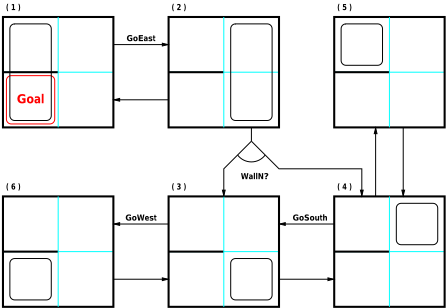
Consider the example of a simple robot navigation domain in Figure 1, containing a 2x2 room with an extra wall. The propositions of the domain are NW, NE, SW, and SE, corresponding to the four positions in the room. Exactly one of them holds in each of the four states in ✌ . The robot can move in the four directions (deterministic actions GoNorth, GoSouth, GoWest and GoEast), provided that there is not a wall in the direction of motion. The action is not applicable, otherwise. At each time tick, the information of walls proximity in each direction is available to the robot (observation variables WallN, WallS, WallW and WallE). For instance, we have that for any action ❀ of the domain ✖ ❘ ❚ ❯ ❯ ❱ ★ ❳ ❩ ☛ ❀ ☛ ✽ ✫ and ✖ ❘ ❚ ❯ ❯ ❘ ★ ❳ ❩ ☛ ❀ ☛ ✻ ✫ . In this case, every observation variable is defined in every state and after the execution of any action of the domain. We call action-independent the observation variables that provide useful information automatically, independently of the previous execution of an action. We require an action-independent observation variable ✤ to satisfy, for any ❀ ❴ ☛ ❀ ❛ ❏ ✏ and any ❁ ❏ ✌ , the following condition: ★ ✖ ❍ ★ ❁ ☛ ❀ ❴ ☛ ✻ ✫ ❜ ✖ ❍ ★ ❁ ☛ ❀ ❛ ☛ ✻ ✫ ✫ ❝ ★ ✖ ❍ ★ ❁ ☛ ❀ ❴ ☛ ✽ ✫ ❜ ✖ ❍ ★ ❁ ☛ ❀ ❛ ☛ ✽ ✫ ✫ In the following, we write ✖ ❍ ✛ ✌ ✯ ✹ ✻ ☛ ✽ ✾ when ✤ is actionindependent. In a different formulation of the domain, an action (e.g. ObsWallE) could be required in order to acquire the value of a corresponding variable (e.g. WallE). In this case, WallE would be defined in any state after the action ObsWallE, and undefined otherwise. Such observation variables are modeled as action-dependent. Action-independent observation variables model "automatic sensing" [Tovey and Koenig, 2000], i.e. information that can always be acquired, as usual in embedded controllers, where a signal from the environment is sampled and acquired at a fixed rate, latched and internally available. Action-dependent observations are used inmost observation-basedapproaches to planning (e.g. [Weld et al., 1998]), where the value of a variable can be observed as the explicit effect of an action, like ObsWallW.

3 Conditional Plans

In partially observable domains, plans need to branch on conditions on the value of observable variables. A plan for a domain ❣ is either the empty plan ❤ , an action ❀ ❏ ✏ , the concatenation ❥ ❴ ❦ ❥ ❛ of two plans ❥ ❴ and ❥ ❛ , or the conditional plan ✤ ❧ ❥ ❴ ✳ ❥ ❛ (read "if ✤ then ❥ ❴ else ❥ ❛ "), with ✤ ❏ ✕ . For the example in Figure 1, a plan that moves the robot from the uncertain initial condition NW or SW, to state SW is GoEast ; ( ❩ ♣ a114 a114 ❳ ❧ ✉ ✈ ✇ ✈ ① ② ③ ✳ ❤ ) ; GoWest. Figure 1 depicts the corresponding execution. The action GoEast is executed first. Notice indeed that in the initial condition all the observation variables would have the same value for both NW and SW: therefore the states are indistinguishable, and it is pointless to observe. After the robot moves east, it is guaranteed to be either in NE or SE. The plan then branches on the value of WallN. This allows the planner to distinguish between state NE and SE: if the robot is in NE, then it moves south, otherwise it does nothing. At this point the robot is guaranteed to be in SE, and can finally move west. This plan is guaranteed to reach SW from any of the initial states, either with three actions (if the initial state is NW), or with two actions (if the initial state is SW).

We define ✖ ❍ ④ ✻ ☛ ❀ ⑤ ⑥ ⑧ ✹ ❁ ❏ ✌ ✳ ✖ ❍ ★ ❁ ☛ ❀ ☛ ✻ ✫ ✾ as the set of states in ✌ where ✤ is true, and ✖ ❍ ④ ✽ ☛ ❀ ⑤ ⑥ ⑧ ✹ ❁ ❏ ✌ ✳ ✖ ❍ ★ ❁ ☛ ❀ ☛ ✽ ✫ ✾ as the set of states in ✌ where ✤ is false. If ✤ is undefined in a state ❁ after ❀ , then ❁ ❏ ✖ ❍ ④ ✻ ☛ ❀ ⑤ ❷ ✖ ❍ ④ ✽ ☛ ❀ ⑤ . In the case of action-independent observations, we have ✖ ❍ ④ ✻ ⑤ ⑥ ⑧ ✹ ❁ ❏ ✌ ✳ ✖ ❍ ★ ❁ ☛ ✻ ✫ ✾ , and ✖ ❍ ④ ✽ ⑤ ⑥ ⑧ ✹ ❁ ❏ ✌ ✳ ✖ ❍ ★ ❁ ☛ ✽ ✫ ✾ . Under partial observability, plans have to work on sets of states whose elements cannot be distinguished, i.e., on "belief states". We say that an action ❀ is applicable to a non empty belief state ❸ ❁ iff ❀ is applicable in all states of ❸ ❁ . We now define plan execution in the case of action-independent observations.

Definition 2 Let ❹ ❺ ⑧ ❸ ❁ ✛ ✌ . The execution of a plan in a set of states is defined as follows:

1. Exec ④ ❥ ⑤ ★ ❹ ✫ ⑥ ⑧ ❹ ; 2. Exec④ ❀ ⑤ ★ ❸ ❁ ✫ ⑥ ⑧ ✹ ❁ ❂ ❻ ✓ ★ ❁ ☛ ❀ ☛ ❁ ❂ ✫ ☛ with ❁ ❏ ❸ ❁ ✾ , if ❀ is applicable in ❸ ❁ ; 3. Exec ④ ❀ ⑤ ★ ❸ ❁ ✫ ⑥ ⑧ ❹ , if ❀ is not applicable in ❸ ❁ ; 4. Exec ④ ❤ ⑤ ★ ❸ ❁ ✫ ⑥ ⑧ ❸ ❁ ; 5. Exec④ ❥ ❴ ❦ ❥ ❛ ⑤ ★ ❸ ❁ ✫ ⑥ ⑧ Exec ④ ❥ ❛ ⑤ ★ Exec ④ ❥ ❴ ⑤ ★ ❸ ❁ ✫ ✫ ; 6. Exec④ ✤ ❧ ❥ ❴ ✳ ❥ ❛ ⑤ ★ ❸ ❁ ✫ ⑥ ⑧ Exec ④ ❥ ❴ ⑤ ★ ❸ ❁ ❷ ✖ ❍ ④ ✻ ⑤ ✫ ❿ Exec ④ ❥ ❛ ⑤ ★ ❸ ❁ ❷ ✖ ❍ ④ ✽ ⑤ ✫ , if (a) if ❸ ❁ ❷ ✖ ❍ ④ ✻ ⑤ ❺ ⑧ ❹ , then Exec④ ❥ ❴ ⑤ ★ ❸ ❁ ❷ ✖ ❍ ④ ✻ ⑤ ✫ ❺ ⑧ ❹ (b) if ❸ ❁ ❷ ✖ ❍ ④ ✽ ⑤ ❺ ⑧ ❹ , then Exec④ ❥ ❛ ⑤ ★ ❸ ❁ ❷ ✖ ❍ ④ ✽ ⑤ ✫ ❺ ⑧ ❹ 7. Exec④ ✤ ❧ ❥ ❴ ✳ ❥ ❛ ⑤ ★ ❸ ❁ ✫ ⑥ ⑧ ❹ otherwise.

We say that a plan ❥ is applicable in ❸ ❁ ❺ ⑧ ❹ iff Exec ④ ❥ ⑤ ★ ❸ ❁ ✫ ❺ ⑧ ❹ . If the plan is applicable, then its execution is the set of all states that can be reached after the execution of the plan. For conditional plans, we collapse into a single set the execution of the two branches (item 6). The conditions (a) and (b) guarantee that both branches are executable. Definition 2 can be extended to the case of action-dependent observations by replacing ✖ ❍ ④ ✻ ⑤ with ✖ ❍ ④ ✻ ☛ ❀ ⑤ and ✖ ❍ ④ ✽ ⑤ with ✖ ❍ ④ ✽ ☛ ❀ ⑤ , where ❀ is the last action executed in the plan. Notice that, at starting time, action-dependent observation variables must be undefined since no action has been previously executed. For lack of space, we omit the explicit formal definition. We formalize the notion of planning problem under partial observability as follows.

Definition 3 (Planning Problem and Solution) A planning problem is defined as a 3-tuple ✟ ➀ ☛ ➂ ☛ ❣ ✘ , where ❣ is a planning domain, ❹ ❺ ⑧ ➀ ✛ ✌ is the set of initial states, and ❹ ❺ ⑧ ➂ ✛ ✌ is the set of goal states. The plan ❥ is a solution to the problem ✟ ➀ ☛ ➂ ☛ ❣ ✘ iff ❹ ❺ ⑧ Exec ④ ❥ ⑤ ★ ➀ ✫ ✛ ➂ .

4 The Planning Algorithm

When planning under partial observability, the search space can be seen as an and-or graph over belief states, recursively constructed from the initial belief state, expanding each encountered belief state by every possible combination of applicable actions and observations. Consider the example in Figure 1, where ➀ is ✹ ➇ ➈ ☛ ➉ ➈ ✾ and ➂ is ✹ ➉ ➈ ✾ . For instance, belief state 1 expands in the or-node [(2)], representing the effect of action GoEast. Other actions are not applicable, and observation conveys no information. Belief state 2 expands in the or-node [(1) (3,4)], representing the effect of action GoWest, resulting in belief state 1, and the effect of observing WallN, resulting in the belief states 3 and 4. In order to find a solution for 2, it is either possible to find a solution for 1, or a solution for both 3 and 4. Non-applicable actions are discarded.

We plan under partial observability by exploring the andor search space described above. The algorithm is basically a postorder traversal of the search space, proceeding forward from the initial belief state, and ruling out cyclic plans. The state of the search is stored by associating a mark to each encountered belief state. Possible marks are NONE, PROCESSING, SOLVED and VISITED, associated to a belief state Bs to

procedure ORSRCH(OrNode) 1 res := ✟ Failure ➌ ➇ ➍ ➎ ✘ ; 2 while(OrNode ❺ ⑧ Nil ❜ ISFAILURE(res)) 3 res := MERGERESULTS(ANDSRCH(first(OrNode)),res); 4 OrNode := rest(OrNode); 5 return res; procedure ANDSRCH(AndNode) 1 res := Success; 2 while(AndNode ❺ ⑧ Nil ❜ ➏ ISFAILURE(res)) 3 res := BSSRCH(first(AndNode)); 4 AndNode := rest(AndNode); 5 return res; procedure BSSRCH(Bs) 1 if (ISBSPROCESSING(Bs)) 2 return ✟ Failure ➌ ★ ❸ ❁ ✫ ✘ ; 3 else if (ISBSSOLVED(Bs)) 4 return Success; 5 else if(ISBSNONE(Bs) ❜ ❸ ❁ ✛ ➂ ) 6 MARKBSSOLVED(Bs); 7 return Success; 8 else 9 PrevFailure := RETRIEVEFAILURE(Bs); 10 if (ISFAILURE(PrevFailure)) 11 return PrevFailure; 12 else 13 MARKBSPROCESSING(Bs); 14 res := ORSRCH(BSEXPAND(Bs)); 15 if (ISFAILURE(res)) 16 MARKBSVISITED(Bs); 17 MEMOIZEFAILURE(Bs,REMOVEBS(res,Bs)); 18 return REMOVEBS(res,Bs); 19 else 20 MARKBSSOLVED(Bs); 21 return Success;

distinguish between the following situations. NONE: Bs has not been previously encountered. SOLVED: a plan has been already found for Bs. PROCESSING: Bs is being processed (i.e. it is currently on the stack). VISITED: Bs has been previously processed, but the search has failed, and currently Bs is not on the stack. If a belief state marked PROCESSING is found, then the search has bumped into a cycle, and shall therefore fail. A VISITED Bs may deserve further expansion (and be therefore marked PROCESSING again). The primitives for recognizing and setting the mark of a belief state are ISBS ✟ MARK ✘ and MARKBS ✟ MARK ✘ .

In order to avoid visiting over and over portions of the search space, we also store previous failures, associating with a belief state the set of belief states that were marked PROCESSING and blocked the search because of cycle detection. We store under which hypothesis did a search attempt fail, with the MEMOIZEFAILURE primitive. Before retrying to process a visited belief state Bs, the data base of failures is accessed with RETRIEVEFAILURE to check if any of the previous failures applies to the current situation, i.e. it is associated to Bs and all of the belief states contained in it are currently being processed. In this case, Bs is not processed, and the retrieved failure is returned.

The planning algorithm is presented in Figure 2. The algorithm is built on 3 recursive subroutines, each returning either Success, to signal that the search completed successfully, or a pair ✟ Failure ➌ reason ✘ , to signal that the search has failed because the belief states in reason are on the stack. (For lack of space, the plan construction steps carried out in case of search success are not reported here but only outlined in the case of the example.) ORSRCH processes an or-node, i.e. a list of and-nodes. And-nodes are repeatedly extracted from the ornode and used as input to ANDSRCH. The results are processed by MERGERESULTS, that constructs the return value by accumulating the set of the failure reasons of the different and searches. If a success is found, then it becomes the return value. Therefore, the search proceeds until a success is found, or the or-node is completely explored, in which case a failure is returned. ANDSRCH processes an and-node, trying to find a solution for each of the contained belief states. It selects the most promising belief state in the and-node, and uses it as input to BSSRCH. As soon as a failed search is detected, a failure-reason pair is propagated. If a success is received for each belief state, then a success is returned. BSSRCH processes a single belief state. It first checks if Bs is a loop back, in which case a failure (due to the Bs itself) is constructed and returned. In lines 3-4, the case of success is handled. In lines 5-7, a node that is encountered for the first time is checked against the goal. Then (lines 8-11), RETRIEVEFAILURE is called to check if Bs can be pruned based on a previous failure. Otherwise, Bs is put on the stack (line 13) and expanded by BSEXPAND, that constructs the corresponding or-node. This is provided in input to ORSRCH. If the result is a failure, then Bs is removed from the stack. The failure is stored disregarding Bs itself (primitive REMOVEBS) since when the search started it was not on the stack. The planner is invoked as BSSRCH ★ ➀ ✫ .

Figure 3 depicts the data structures built by the algorithm while solving the example problem of Figure 1. For each step, we report the belief states marked PROCESSING and marked VISITED, the stored failures, the belief states marked SOLVED and the associated plan. Failure 5(4), introduced at step 6, means that the search started on belief state 5 failed because of a loop back on ➞ that was PROCESSING. The last column associates the plan ❥ ➟ to each belief state ➍ becoming SOLVED. Belief state 6 is a subset of ➂ and is thus associated with the empty plan. ❥ ➠ is the concatenation of the action GoW, that leads from 3 to 6, with ❥ ➡ . The case for ❥ ➢ is similar. The conditional plan ❥ ❛ is constructed by ANDSRCH: the observation variable WallN associated with the and-node (3,4) being manipulated is the test of the plan, while the branches are the plans ❥ ➠ and ❥ ➢ associated to the successful belief states 3 and 4. Notice that belief state 4 is processed again at step 11, after the failure due to the loopback on 3 at step 7. The storage of previous failures can speed up the search substantially, e.g., if fromNW it were possible to enter in a different "branch" of the navigation domain that cannot lead to the solution.

5 The Planner

We integrated the algorithm described above in MBP [Cimatti et al., 1998], a planner for nondeterministic domains based on Binary Decision Diagrams (BDD) [Bryant, 1992] and symbolic model checking techniques [McMillan, 1993]. MBP allows for conditional planning under full observability [Cimatti et al., 1998], also considering temporally extended goals [Pistore and Traverso, 2001]. For this work, we extended MBP in two main directions. First, we developed a BDD-based implementation for the observation relation ✖ . Second, we implemented the search algorithm described in previous section. We rely on the machinery of [Bertoli et al., 2001], where conformant planning is tackled as deterministic (rather than and-or) search in the space of belief states. Each visited belief state is represented by a unique BDD, while a hashing structure is used to efficiently implement the marking mechanism described in previous section. The expansion of a belief state ❸ ❁ (primitive BSEXPAND) can be described in logical terms, and is implemented by means of BDD-based transformations. We first apply the symbolic expansion used in the case of conformant planning that computes the belief states corresponding to the execution from ❸ ❁ of all the possible actions. Then, for each of the generated belief states ❸ ❁ ➟ , we take into account the effect of observations by generating, for each ✤ , the and-nodes of the form ★ ❸ ❁ ➟ ❷ ✖ ❍ ④ ✻ ⑤ ☛ ❸ ❁ ➟ ❷ ✖ ❍ ④ ✽ ⑤ ✫ . However, in order to dominate the complexity of the application of the full combination of observations, we apply the following automatic, domainindependent simplifications. First, we analyze the domain to discover if it is possible to consider only one observation at a time without losing completeness. When this is not possible, we apply observations "set-wise" to ❸ ❁ , i.e. if we consider ✤ ➟ and ✤ ➤ , the corresponding splits are both applied, resulting in the and-node ★ ❸ ❁ ➟ ❷ ✖ ❍ ➦ ④ ✽ ⑤ ❷ ✖ ❍ ➨ ④ ✽ ⑤ ☛ ❸ ❁ ➟ ❷ ✖ ❍ ➦ ④ ✽ ⑤ ❷ ✖ ❍ ➨ ④ ✻ ⑤ ☛ ❸ ❁ ➟ ❷ ✖ ❍ ➦ ④ ✻ ⑤ ❷ ✖ ❍ ➨ ④ ✽ ⑤ ☛ ❸ ❁ ➟ ❷ ✖ ❍ ➦ ④ ✻ ⑤ ❷ ✖ ❍ ➨ ④ ✻ ⑤ ✫ . In general, plans may be produced where the same observations are needlessly carried out on all branches, or useless actions precede observations. A special purpose procedure postprocesses the solution, getting rid of these sources of redundancy. Finally, the and-or search is driven by a simple selection heuristic that orders the or-node by delaying the expansion of the belief states where no observation has effect.

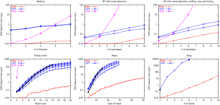
fied). The results of the comparison are depicted in Table 1. Each plot refers to a problem class. We report on a logarithmic scale the search time (in seconds). The performance of SGP tends to degrade quite rapidly. The instances of BT with 8 packages reached the time limit. In the case of empty room, SGP was unable to solve the 3x3 version of the problem in 12 hours of CPU time. For GPT we report the average performance (over 10 runs) on increasing numbers of trial runs. In order to ensure a fair comparison, we would have liked to report the performance of GPT on the minimum number of trials needed for convergence. Unfortunately, detecting whether GPT has converged to a solution is not evident from the output. A necessary condition for convergence appears to be the existence of a successful trial for each possible initial state: therefore, the cardinality of the initial state (called ➫ in the following) is a lower bound for convergence. The reported results correspond to increasing multiples of ➫ (the computation time grows accordingly). As one increases the number of trials, the probability of GPT converging to a solution increases. For simpler problems like Medical and BT, GPT converges after a small number of trial runs. However, in the more complex problems, the number of initial states increases, as well as the required number of trials. This implies a growth of the computational resources needed, as clear from the results. For the Maze tests, the parser was unable to deal with problems larger than 29. For the Ring(6) domain, GPT fails to compute the heuristic function within the time limit. We tried to run it without heuristics, but it exhausted the available memory after 3 hours of CPU time. A very important point is that the difficulty of the problem slows down convergence, due to increasing possibility of failed and/or repeated trials upon certain initial states. The thick line with bullets, crossing the results of GPT, indicates up to which problem size GPT reached convergence at least once. For instance, in the empty roomdomain, GPT did not find a solutionwith ➞ ➭ ➫ for room size larger than 14 in any of the attempted 10 runs.

6 Experimental Evaluation

We experimentally evaluated our approach against SGP [Weld et al., 1998] and GPT [Bonet and Geffner, 2000]. (Other similar systems, e.g. CASSANDRA [Pryor and Collins, 1996], that are outperformed by SGP, as shown in [Weld et al., 1998], are not considered.) SGP is based on GRAPHPLAN. It produces acyclic conditional plans, but it is unable to deal with nondeterministic action effects, i.e. uncertainty is limited to the initial condition. A planning graph is built for each initial state that can be distinguished by observation. GPT models planning domains as Markov Decision Processes, and, based on the probability distributions, produces a policy associating actions to belief states. The search is based on the repeated generation of learning/control trials, starting from randomly selected states in the initial belief state. The policy tends to improve as the number of trials grows. GPT cannot guarantee that the returned policies are acyclic.

We considered several test domains. The ones from the distributions of SGP turned out to be trivial, and therefore we report only the results for Medical and BT (see [Weld et al., 1998] for a description). The Maze domains [Tovey and Koenig, 2000] are similar to the explanatory example in Figure 1, where a certain goal position has to be reached from a completely unknown initial position. The Empty room problem is basically a maze without internal walls. The Ring domain [Cimatti and Roveri, 2000] is a ring-shaped navigation domain, where each room has a window that the robot can observe and open/close. The goal is to have all windows closed, while the initial situation is unknown. We did not consider some of the domains from the GPT distribution. Some of these are meaningful only in a probabilistic setting, or admit only cyclic solutions (e.g. the Omelette domain).

The experiments were run on a Pentium II 300MHz with 512Mb of memory running Linux, fixing a memory limit of 500Mb and timeout to 1 hour CPU (unless otherwise speci- Similarly for the mazes with size larger that 15. MBP tackles the analyzed problems quite well. Search in the belief space avoids the explosion following from the enumeration of initial states, while the use of symbolic data structures limits memory requirements. The produced plans are of reasonable length, with the exception is the ring domain, where the selection function is not effective: combined with the depth-first search of the algorithm, this results in extremely intricated plans. Further research is needed to tackle this problem.

7 RelatedWork and Conclusions

In this paper we have presented a novel approach to conditional planning under partial observability. The approach is based on a model of observation that encompasses automatic sensing [Tovey and Koenig, 2000] and action-based sensing [Cassandra et al., 1994; Weld et al., 1998; Bonet and Geffner, 2000]. See also [Goldman and Boddy, 1996] for a similar model of observation. The planning algorithm is based on the exploration of a (possibly cyclic) and-or graph induced by the domain. It is different from heuristic search algorithms like AO*, that are based on the assumption that and-or search graphs are acyclic. Given the exhaustive style of the exploration, the algorithm can decide whether the problem admits an acyclic solution, i.e. a plan guaranteed to reach the goal in a finite number of steps. The algorithm is efficiently implemented in the MBP planner by means of BDD-based symbolic model checking techniques. We show that MBP outperforms the SGP and GPT planners. Another interesting system is QBFPLAN [Rintanen, 1999a], that extends the SAT-based approach to planning to the case of nondeterministic domains. The planning problem is reduced to a QBF satisfiability problem, that is then given in input to an efficient solver [Rintanen, 1999b]. QBFPLAN relies on a symbolic representation, but the approach seems to be limited to plans with a bounded execution length. The search space is significantly reduced by providing the branching structure of the plan as an input to the planner.

The problem of planning under partial observability has been deeply investigated in the framework of Partially Observable MDP (see, e.g., [Cassandra et al., 1994; Hansen and Zilberstein, 1998; Poupart and Boutilier, 2000]). GPT follows this approach. Methods that interleave planning and execution [Koenig and Simmons, 1998; Genesereth and Nourbakhsh, 1993] can be considered alternative (and orthogonal) approaches to the problem of planning off-line with large state spaces. However, these methods cannot guarantee to find a solution, unless assumptions are made about the domain. For instance, [Koenig and Simmons, 1998] assumes "safely explorable domains" without cycles. [Genesereth and Nourbakhsh, 1993] describes an off-line planning algorithm based on a breadth-first search on an and-or graph. The paper shows that the version of the algorithm that interleaves planning and execution is more efficient than the off-line version, both theoretically and experimentally.

Future research objectives are the extension of the partially observable approach presented in this paper to strong cyclic solutions [Cimatti et al., 1998] and for temporally extended goals [Kabanza et al., 1997]. We will also investigate the use of heuristic search techniques, and the extension to the case of planning with non-deterministic/noisy sensing.