Observation Reduction for Strong Plans

1 Introduction

In recent years, increasing interest has been devoted to planning in non-deterministic domains. Strong planning (i.e. finding automatically a plan which is guaranteed to achieve the goal regardless of nondeterminism) is an important problem in this research field. Under full observability or partial observability, this problem has been addressed in the literature: in the frame for full observability proposed in [Cimatti et al., 1998b; 2003], a plan is a state-action table; in the frame for partial observability proposed in [Bertoli et al., 2001; 2006], a plan is a conditional plan branching on the values of observation variables.

The cases of full observability, see e.g., [Cimatti et al., 1998b; 2003], where the whole status of the domain is observed at every step, and the cases of partial observability, see e.g., [Boutilier, 2002; Eiter et al., 2003; Herzig et al., 2003; Bertoli et al., 2001; 2006], where the plan executor cannot access the whole status of the domain, are both under the assumption that the set of observation variables is fixed and compulsory. In real world domains (e.g., many robotics, control, and scheduling domains), however, observation variables are optional and many of them are useless in the executions of the plans; on the other side, information acquisition may require some kind of cost (e.g. time, money, and power etc.). So it is significant to find a minimal set of observation variables that are necessary for the execution of a plan, and to best of our knowledge, it is still an open problem.

In this paper we present a first attempt to solve the problem. Under the hypothesis that any two distinct states of the domain can be distinguished by an observation variable at least, we define an algorithm that finds an approximate minimal set (written as Vobs) of observation variables that are necessary for the execution of a strong plan under full observability (i.e. a state-action table), and transforms the plan into a strong plan under partial observability (i.e. a conditional plan branching on the observations built on Vobs). This algorithm first exploits the belief state [Bonet and Geffner, 2000] (i.e. the set of possible current states) at every step to compute Vobs; then, it transforms the given state-action table into a conditional plan branching on the observations built on Vobs. The algorithm is based on the frameworks for strong planning under full observability proposed in [Cimatti et al., 2003] and partial observability proposed in [Bertoli et al., 2006].

The paper is organized as follows. We first recap the frameworks proposed in [Cimatti et al., 2003] and [Bertoli et al., 2006] (Section 2); then, we introduce the key notions of the algorithm and describe the algorithm in detail (Section 3); finally, Section 4 draws some conclusions and discusses future research directions.

2 Domains, Observations, Plans, and Problems

In this section, we briefly review some definitions of strong planning in non-deterministic domains under full observability and partial observability that are relevant to our work. Further details and examples of these definitions can be found in [Cimatti et al., 2003; Bertoli et al., 2006].

A planning domain is a model of a generic system with its own dynamics.

Definition 1 A planning domain is a tuple Σ = 〈S,A,R〉, where S is a finite set of states, A is a finite set of actions, and R : S × A → 2S is the transition function. The transition function associates to each state s ∈ S and to each action a ∈ A the set R(s, a) ⊆ S of next states.

The set of actions that are applicable in state s is ACT(s) = {a|∃s′ ∈ R(s, a)}.

In practice, a domain may have many observation variables, whose value can be observed at run-time.

Definition 2 Let Σ = 〈S, A, R〉 be a planning domain. Let V be a finite set of observation variables. An observation function over S and V is a function X : S × V → {⊤, ⊥}.

From Definition 2, for each state, there is a corresponding complete set of assignments to observation variables.

Plans can control the evolutions of the domain by triggering actions. A plan under full observability is a set of stateaction pairs.

Definition 3 A plan πF for Σ is a set of pairs 〈s, a〉 (i.e. a state-action table), where: s ∈ S, a ∈ ACT(s), and there is at most one action a such that 〈s, a〉 ∈ πF for any state s.

The execution of a state-action table πF in Σ can be represented as execution structure, i.e. a directed graph in which the nodes are all of the states of the domain that can be reached by executing actions in the state-action table, and the arcs represent possible state transitions caused by actions in πF .

Definition 4 Let πF be a state-action table for Σ. The execution structure induced by πF from the set of initial states I ⊆ S is a tuple K = 〈Q, T 〉, where Q ⊆ S and T ⊆ S ×S are the minimal sets satisfying the following rules:

1. if s ∈ I, then s ∈ Q, and
2. if s ∈ Qand there exists a state-action pair 〈s, a〉 ∈ πF such that s′ ∈ R(s, a), then s′ ∈ Q and T (s, s′ ).

A state s ∈ Q is a terminal state of K if there is no s′ ∈ Q such that T (s, s′ ). A path of K from s0 ∈ I is a possibly infinite sequence s0, s1, . . . of states in Q such that, for every state si in the sequence, either si is the last state of the sequence (in which case si is a terminal state of K) or T (si, si+1) holds.

A planning problem for a given domain is described by a set of possible initial states, and a set of goal states.

Definition 5 Let Σ = 〈S,A,R〉 be a planning domain. A planning problem for Σ is a triple P = 〈Σ, I, G〉, where I ⊆ S and G ⊆ S.

In the following discussion, Σ = 〈S,A,R〉, V, X, P = 〈Σ, I, G〉, πF , and K represent a planning domain, a finite set of observation variables, an observation function over S and V, a planning problem for Σ, a state-action table for Σ, and the execution structure induced by πF from I, respectively.

In many cases, we are interested in strong solutions to P, i.e. plans that are guaranteed to achieve the goal in spite of nondeterminism.

Definition 6 πF is a strong solution to P if K is acyclic and all terminal states of K are in G.

In fact, any state-action table πF for Σ is a strong solution to some planning problems for Σ, if its execution structure K is acyclic and all terminal states of K are in G. So in the following discussion, we use interchangeably the terms strong solution and strong plan.

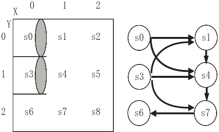
In the following example, we illustrate the definitions given in this section.

Example 1 A simple robot navigation domain Σ is shown on the left of Figure 1. The robot can be in nine positions of a room, corresponding to the states of the domain: S = {s0, . . . , s8}. It can move in the four directions, corresponding to actions A = {GoNorth, GoSouth, GoEast,GoWest}. An action is applicable only if there is no wall in the direction of motion, e.g. R(s0,GoSouth) = ∅. All the actions are deterministic (e.g., R(s7,GoWest) = {s6}), except for action GoEast when on s0 (or s3), where the robot may slip and end up either in s1 or s4 (or in s1, s4, or s7), i.e. R(s0,GoEast) = {s1, s4} and R(s3,GoEast) = {s1, s4, s7}. Let I = {s0, s3} and G = {s6}. Then πF = {〈s0,GoEast〉, 〈s1,GoSouth〉, 〈s3,GoEast〉, 〈s4,GoSouth〉, 〈s7,GoWest〉} is a strong plan to P = 〈Σ, I, G〉, and its execution structure K is shown on the right of Figure 1.

Suppose that the sensors of the robot can detect walls in the current position. This can be formalized with four observation variables, i.e. WallN, WallS, WallW and WallE. In addition, there are six responders (i.e. X0, X1, X2, Y0, Y1, and Y2) located at the north or west border of the room. They work as the X-axis and Y-axis of the nine positions (let 1 ≤ n ≤ 3):

1. The robot sends n pulses north (or west) via the ground.
2. If the responder Xn-1 (or Yn-1) receives n pulses then it sends a responsive pulse south (or east), else it does nothing.
3. The robot can detect whether its X-coordinate (or Ycoordinate) is n by receiving a responsive pulse or not in a appointed time.

This can be formalized with six observation variables, i.e. X0, X1, X2, Y 0, Y 1 and Y 2. So the set of observation variables V is {WallN, WallS, WallW, WallE, X0, X1, X2, Y 0, Y 1, Y 2}; and the observation function X is such that X (s0, WallE) = ⊥, X (s2, X2) = ⊤, and so on.

3 Observation Reduction for Strong Plans

In most real world domains, observation variables are optional and many of them are useless in the execution of a plan (e.g. consider the situation represented in Example 1, the responder X2 can be turned off before the execution of πF ); on the other side, information acquisition may require some kind of cost (e.g. time, money, and power etc.). So it is significant to find a minimal set of observation variables which are necessary for the execution of a plan.

In this paper, it is assumed that any two distinct states of the domain can be distinguished by an observation variable at least. So state-action tables are acceptable at execution level. In the execution of a state-action table πF , the executor is required to observe the values of all the observation variables; consequently, it can know what the current state is and execute the appropriate action at every step. But in many cases, there is much observation information that is useless in the execution of a plan. For example, it makes no sense to observe the value of an observation variable v, where X(s, v) = ⊤ (or X(s, v) = ⊥) for any possible current state s (hereafter, B denotes the set of possible current states, i.e. the current belief state); and there is no need to do any detection if there exists a ∈ A such that 〈s, a〉 ∈ πF for any s ∈ B.

In this section, we define an algorithm that finds an approximate minimal set of observation variables (i.e. Vobs) which are necessary for the execution of a strong plan, and transforms the strong plan into a conditional plan branching on the observations built on these observation variables. Before explaining the algorithm in detail, we introduce some notions used in it.

In the execution of πF , the action that should be executed on s is written as ACTION(s, πF). That is to say, if ∃a ∈ A. 〈s, a〉 ∈ πF then ACTION(s, πF) = a, else ACTION(s, πF ) = nop (nop means doing nothing).

Let ∅ ⊂ Vobs ⊆ V. For each s ∈ S, we represent the corresponding set of assignments to the observation variables of Vobs with CODE(s, Vobs, X ), where:

• if Vobs = {v} and X(s, v) = ⊤, then CODE(s, Vobs, X ) = v.
• if Vobs = {v} and X(s, v) = ⊥, then CODE(s, Vobs, X ) = ¬v.
• if |Vobs| > 1 and v ∈ Vobs, then CODE(s, Vobs,X) = CODE(s, {v},X) ∧ CODE(s, Vobs - {v}, X ).

The above representation naturally extends to any ∅ ⊂ Q ⊆ S as follows:

The set of observations built on V and X is O(V,X) = {CODE(Q, Vobs, X) | ∅ ⊂ Q ⊆ S, ∅ ⊂ Vobs ⊆ V}.

The definition of conditional plans branching on O(V, X) is given as follows. In fact, it is an extension of the one proposed in [Bertoli et al., 2006].

Definition 7 The set of conditional plans Π for 〈Σ, V,X〉 is the minimal set such that:

• ε ∈ Π, ε is the empty plan;
• if a ∈ A and π ∈ Π, then a ◦ π ∈ Π;
• if o ∈ O(V,X), and π1, π2 ∈ Π, then if o then π1 else π2 ∈ Π.

In general, we are interested in applicable plans, i.e. plans whose execution guarantees that an action is never attempted unless it is applicable, regardless of nondeterminism.

Definition 8 A plan π for 〈Σ, V, X〉 is applicable in state s iff either

• π is the empty plan ε; or
• π is a ◦ π′ , a is applicable in s, and π′ is applicable in every s′ ∈ R(s, a); or
• π is if o then π1 else π2, and:
• if the formula CODE(s, V,X) → o is a tautology, π1 is applicable in s; and
• if the formula CODE(s, V,X) →¬o is a tautology, π2 is applicable in s.

The execution of a conditional plan is defined in terms of the runs associated to it. Intuitively, a run contains the states, observations and actions encountered while executing the plan.

Definition 9 A run is a sequence σ = (s0, o0) ◦ a1 ◦ (s1, o1) ◦ . . . ◦ an ◦ (sn, on), where si ∈ S, oi ∈ O(V,X), and ai ∈ A. A sequence σ is a run of π (π is a conditional plan for〈Σ, V, X〉) from state s iff either

• π = ε, and σ = (s, o) with o = CODE(s, V, X); or
• π = a ◦ π1 and σ = (s, o) ◦ a ◦ σ1 with o = CODE(s, V,X), and σ1 is a run for π1 from some s1 ∈ R(s, a) ̸= ∅; or
• π = if o then π1 else π2, CODE(s, V,X) → o is a tautology, and σ is a run of π1 starting from (s, CODE(s, V, X )); or
• π = if o then π1 else π2, CODE(s, V,X) → ¬o is a tautology, and σ is a run of π2 starting from (s, CODE(s, V, X )).

In the following, we write RUNS(s, π) to denote the set of runs of π starting from s. We write FINALSTATES(s, π) to indicate the set of the final states of the runs of RUNS(s, π).

The definition of strong plans to 〈P, V, X〉 is given as follows. In fact, it is similar to the one proposed in [Bertoli et al., 2006].

Definition 10 A conditional plan π for 〈Σ, V, X〉 is a strong plan to 〈P, V, X〉 iff

• π is applicable in every state of I, and
• every run of π from a state in I ends in G, i.e. ⋃s∈I FINALSTATES(s, π) ⊆ G.

Now we can introduce the algorithm for observation reduction of strong plans in detail.

The basic algorithm (i.e. STRONG-FO-PO) is presented in Figure 2. Given a planning problem P, a strong plan πF to P, a finite set of observation variables V, and an observation function X, the algorithm transforms πF into a strong plan

1. function STRONG-FO-PO(P, πF , V,X) 2. dis ← FINDSTATEPAIRS(P, πF ); 3. Vobs ←REDUCTION(dis, V,X); 4. return TRANSFORM(P, πF , Vobs, X ); 5. end

1. function FINDSTATEPAIRS(P, πF ) // Suppose P = 〈Σ, I, G〉 2. parts ← DIVIDE(I, πF ); 3. if (parts = ∅) then 4. return ∅; 5. fi; 6. dis ← ∅; 7. for each (a, Q) ∈ parts 8. Inext ← EXECUTE(Σ, Q, a); 9. P ′ ← 〈Σ, Inext, G〉; 10. dis ← dis ∪ FINDSTATEPAIRS(P ′ , π); 11. endfor; 12. if (I ∩ G ̸= ∅) then 13. parts ← parts ∪ {(nop, I ∩ G)}; 14. fi; 15. for any (a1,Q1), (a2,Q2) ∈ parts, where a1 ̸= a2 16. for any s1 ∈ Q1, s2 ∈ Q2 17. dis ← dis ∪ {(s1, s2)}; 18. endfor; 19. endfor; 20. return dis; 21. end

to 〈P, Vobs, X〉, where Vobs is an approximate minimal set of observation variables which are necessary for the execution of πF . The STRONG-FO-PO algorithm has two main phases: (1) an observation reduction phase (lines 2-3), in which Vobs is computed by applications of FINDSTATEPAIRS and REDUCTION, and (2) a transform phase (line 4), in which πF is transformed into a conditional plan for 〈Σ, Vobs, X〉 by an application of TRANSFORM.

In order to compute Vobs, we calculate dis ⊆ S × S: if (s1, s2) ∈ dis, then {s1, s2} ⊆ B (i.e. the set of possible current states) at some step of the execution of πF and ACTION(s1, πF ) ̸= ACTION(s2, πF). This task is accomplished by the FINDSTATEPAIRS procedure, which is presented in Figure 3.

Now let us introduce the FINDSTATEPAIRS procedure in detail:

• First (line 2), the set of possible current states (i.e. I) are divided into some divisions according to the actions specified by πF . The partition is realized through the function DIVIDE. Formally, DIVIDE(I, πF ) = {(a, Q) | a ∈ A, ∅ ⊂ Q ⊆ I, s ∈ Q iff 〈s, a〉 ∈ πF }.
• Second (lines 3-5), if parts = ∅ (i.e. I ⊆ G), then an

1. function REDUCTION(dis, V,X) // Suppose V = {v1, . . . , vn} 2. for n ≥ i ≥ 1 do di[i] ← 0; 3. for all (s1, s2) ∈ dis 4. for n ≥ i ≥ 1 5. if (X(s1, vi) ̸= X(s2, vi)) then 6. di[i] ← di[i] + 1; 7. fi; 8. endfor; 9. endfor; 10. Vobs ← ∅; 11. while (dis ̸= ∅) 12. let di[i] = max{di[k] | n ≥ k ≥ 1}; 13. Vobs ← Vobs ∪ {vi}; 14. for all (s1, s2) ∈ dis 15. if (X(s1, vi) ̸= X(s2, vi)) then 16. delete (s1, s2) from dis; 17. fi; 18. endfor; 19. di[i] ← 0; 20. endwhile; 21. return Vobs; 22. end

empty set is returned by FINDSTATEPAIRS.

• Third (lines 6-11), the elements of dis corresponding to the next belief state are computed by simulating the strong plan's execution for one step and an application of FINDSTATEPAIRS itself. The simulation of a plan is realized through the function EXECUTE. Formally, EXECUTE(Σ, Q, a) = ⋃s∈Q R(s, a).
• Finally (lines 12-19), if the actions specified by πF for I are not consistent (i.e. |parts| > 1), then any two states (e.g. s1 and s2) from different divisions of I should be distinguished from each other, i.e. (s1, s2) or (s2, s1) should be included in dis if a1 ̸= a2, (a1,Q1) ∈ parts, (a2, Q2) ∈ parts, s1 ∈ Q1, and s2 ∈ Q2.

Figure 4 shows the REDUCTION procedure. Given dis ⊆ S ×S, V, and X as input, the REDUCTION procedure returns an approximate minimal set of observation variables Vobs such that ∀(s1, s2) ∈ dis. ∃v ∈ Vobs.X(s1, v) ̸= X(s2, v). It starts with Vobs = ∅ and iteratively adds some v ∈ V into Vobs until d = dis, where d = {(s1, s2) ∈ dis | ∃v ∈ Vobs. X(s1, v) ̸= X(s2, v)}.

The TRANSFORM procedure is presented in Figure 5. Its role is to transform πF (i.e. a strong plan to P) into a strong plan π to 〈P, Vobs, X〉.

Now let us introduce the TRANSFORM procedure in detail. At first (line 2), the belief state (i.e. I) is divided into some divisions according to the actions specified by πF . The partition is realized through the function DIVIDE. And then:

1. If I ⊆ G (lines 3-4), then an empty plan ε is returned.
2. Else if I ∩ G ̸= ∅ (lines 5-8), then if o then ε else TRANSFORM(P ′ , πF , Vobs, X) is returned, where:

1. function TRANSFORM(P, πF , Vobs,X) // Suppose P = 〈Σ, I, G〉 2. parts ← DIVIDE(I, πF ); 3. if I ⊆ G then 4. return ε; 5. else if I ∩ G ̸= ∅ then 6. o ←MAKECODE(I ∩ G, I - G, Vobs, X ); 7. P ′ ← 〈Σ, I - G, G〉; 8. return if o then ε else TRANSFORM(P ′ , πF , Vobs, X ); 9. else if parts = {(a,Q)} then // i.e. |parts| = 1 10. Inext ←EXECUTE(Σ, Q, a); 11. P ′ ← 〈Σ, Inext, G〉; 12. return a ◦ TRANSFORM(P ′ , πF , Vobs, X ); 13. else 14. select an element (a,Q) from parts; 15. o ←MAKECODE(Q, I - Q, Vobs, X ); 16. P ′ ← 〈Σ, Q, G〉, P ′′ ← 〈Σ, I - Q, G〉; 17. return if o then TRANSFORM(P ′ , πF , Vobs, X) else TRANSFORM(P ′′ , πF , Vobs, X ); 18. fi; 19. end

• o is an observation that can distinguish the states in I ∩ G from the states in I - G.
• P ′ = 〈Σ, I - G, G〉.

o is computed by MAKECODE(I ∩ G, I - G, Vobs, X). Figure 6. shows the MAKECODE subroutine. Given Q1 ⊆ S, Q2 ⊆ S, Vobs, and X as input, the MAKECODE subroutine finds an approximate minimal set of observation variables Vnow ⊆ Vobs such that ∀(s1, s2) ∈ Q1 × Q2. ∃v ∈ Vnow.X(s1, v) ̸= X(s2, v), and returns the observation of Q1 built on Vnow and X (i.e. CODE(Q1, Vnow, X )).

1. Else if the actions specified by πF for I are consistent, i.e. |parts| = 1 (lines 9-12), then a ◦ TRANSFORM(P ′ , πF , Vobs, X) is returned, where:
2. a is the action specified by πF for all the possible current states.
3. P ′ = 〈Σ, Inext, G〉. Inext is the belief state at next step, and it is computed by EXECUTE(Σ,Q, a).
4. Else (lines 13-17) (a,Q) is selected from parts, and if o then π1 else π2 is returned, where:
5. o is an observation that can distinguish the states in Q from the states in I -Q, and it is computed by MAKECODE(Q, I - Q, Vobs, X ).
6. π1 =TRANSFORM(〈Σ,Q, G〉, πF , Vobs,X).
7. π2 =TRANSFORM(〈Σ, I - Q, G〉, πF , Vobs, X ).

From Definition 6, Definition 10 and the algorithms presented above, we can get Theorem 1 and Theorem 2.

Theorem 1 If πF is a strong plan to P, then STRONG-FO-PO(P, πF , V, X ) terminates.

1. function MAKECODE(Q1,Q2, Vobs,X) 2. dis ← ∅; 3. for any s1 ∈ Q1, s2 ∈ Q2 4. dis ← dis ∪ {(s1, s2)}; 5. endfor; 6. Vnow ← REDUCTION(dis, Vobs,X); 7. return CODE(Q1, Vnow, X ); 8. end

In fact, Theorem 1 can be proved by showing that all the paths of the execution structure K induced by πF from I are finite. According to Definition 6, all the paths of K are finite (i.e. K is acyclic) because πF is a strong plan to P.

Theorem 2 Let πF be a strong plan to P. Let Qt be the set of terminal states of K (i.e. the execution structure induced by πF from I). Suppose π is the conditional plan returned by STRONG-FO-PO(P, πF , V, X). Then:

• π is a strong plan to 〈P, V, X〉, and
• ⋃s∈I FINALSTATES(s, π) = Qt ⊆ G.

In the following example, we illustrate the algorithms described in this section.

Example 2 Consider the situation depicted in Example 1. We apply STRONG-FO-PO to (P, πF , V,X). Firstly, dis is computed by FINDSTATEPAIRS(P, πF), and it is {(s1, s7), (s4, s7)}; and then, Vobs is computed by REDUCTION(dis, V,X), and it is {WallS}; lastly, π is returned by TRANSFORM(P, πF , Vobs, X ), where:

• π = π0 =GoEast ◦ π1, and
• π1 = ifWallS then (GoWest ◦ ε) else π2, and
• π2 =GoSouth ◦ π3, and
• π3 = ifWallS then (GoWest ◦ ε) else π4, and
• π4 =GoSouth ◦ GoWest ◦ ε.

It is easy to find that π is a strong plan to 〈P, V, X〉, and G = ⋃s∈I FINALSTATES(s, π) = {s6} (i.e. the set of terminal states of the execution structure induced by πF from I).

In fact, the observation variables of V-Vobs are useless in the whole executions of π and πF . So the sensors and the responders that correspond to these observation variables (i.e. WallN, WallW, WallE, X0, X1, X2, Y 0, Y 1, and Y 2) can be turned off before executing π. Furthermore, it is not necessary to observe all the values of observation variables of Vobs at every step: for instance, π requires the plan executor to execute GoEast at first, regardless of the observation information about the current state.

4 Conclusions

This paper presents an algorithm (i.e. STRONG-FO-PO) for observation reduction of strong plans under full observability, which take the form of state-action tables. To the best of our knowledge, no other work has discussed and tackled this problem.

Given a planning problem P = 〈Σ, I, G〉, a strong plan πF to P, a finite set of observation variables V, and an observation function X as input, the STRONG-FO-PO algorithm finds Vobs, i.e. an approximate minimal set of observation variables which are necessary for the execution of πF , and transforms πF into a conditional plan π branching on the observations built on Vobs and X, such that:

• π is a strong plan to 〈P, Vobs, X〉, and
• ⋃s∈I FINALSTATES(s, π) = Qt ⊆ G, where Qt is the set of terminal states of the execution structure induced by πF from I.
• The STRONG-FO-PO algorithm always terminates. In the STRONG-FO-PO algorithm, there are two levels of the meaning of observation reduction:
• The observation variables which are useless in the whole execution of a plan πF , are discarded as more as possible. That is to say, the algorithm computes Vobs and discards the observation variables of V - Vobs.
• At every step of the execution of πF , values of the observation variables that are useless in choosing the appropriate action, are discarded as more as possible. That is to say, the algorithm computes Vnow (see Figure 6, line 6) for every step of the execution of πF , and discards the values of observation variables of Vobs - Vnow temporarily.

In the future, we plan to extend this work along the following directions.

• We will investigate the problem under the situation that:
• observation variables may relate to different data types (symbolic, numeric, ordinal, etc.), and
• noisy observations or missing values may be allowed.
• Considering the costs corresponding to observation variables may be different, we will investigate the problem of observation reduction for some plans, in which some preferences should be taken into account.
• We will investigate observation reduction for plans to other kinds of planning problems, in particular strong cyclic planning problems [Cimatti et al., 1998a; Daniele et al., 1999], and planing problems for temporally extended goals [Pistore and Traverso, 2001; Lago et al., 2002].