A Fast Analytical Algorithm for Solving Markov Decision Processes with Real-Valued Resources

1 Introduction

Recent advances in robotics have made aerial, underwater and terrestrial unmanned autonomous vehicles possible. In many domains for which such unmanned vehicles are constructed, the vehicles have to construct plans that obey deadlines or, more generally, resource limits for real-valued resources whose consumption can only be characterized by probability distributions, such as execution time or battery power. It is a major challenge for AI research to construct good plans for these domains efficiently [Bresina et al., 2002]. One cannot model the resulting planning problems with generalized semi-Markov decision processes [Younes and Simmons, 2004] since they can model actions that consume real-valued amounts of resources but not resource limits. One could model them with Markov decision processes (MDPs) by encoding the available amounts of resources in the states. The resulting continuous state MDP can then be solved approximately by discretizing the state space (for example, by discretizing the probability distributions) and then applying standard dynamic programming algorithms, such as value iteration [Boyan and Littman, 2000]. A major drawback of this approach is that discretizing the state space results in a combinatorial explosion of the number of states as the discretization becomes more and more fine-grained. In response, discretization-free approaches have been developed, some of which do not provide strong guarantees on the quality of the resulting policy [Lagoudakis and Parr, 2003; Nikovski and Brand, 2003; Hauskrecht and Kveton, 2003]. Lazy Approximation [Li and Littman, 2005] is currently the leading discretization-free algorithm for solving continuous state MDPs with quality guarantees. It solves the planning problems by approximating the probability distributions over the resource consumptions with piecewise constant functions. It then uses value iteration to solve the resulting MDPs by repeatedly approximating the value functions with piecewise constant value functions. Lazy Approximation has two problems that increase its runtime: First, complex piecewise constant functions are often necessary to approximate probability distributions closely. Second, the value functions need to be reapproximated after every iteration. We thus present CPH (Continuous state MDPs through PHase-type probability distributions), a novel solution method that solves the planning problems by first approximating the probability distributions over the resource consumptions with phase-type distributions, which use exponential distributions as building blocks [Neuts, 1981]. It then uses value iteration to solve the resulting MDPs by exploiting properties of exponential distributions to calculate the value functions after every iteration accurately (= without reapproximations) and efficiently. CPH shares with Lazy Approximation that it provides strong guarantees on the quality of the resulting policy but runs substantially faster than Lazy Approximation in our experimental feasibility study in a Mars rover domain.

∗This material is based upon work supported by the DARPA/IPTO COORDINATORS program and the Air Force Research Laboratory under Contract No. FA875005C0030. The views and conclusions contained in this document are those of the authors and should not be interpreted as representing the official policies, either expressed or implied, of the Defense Advanced Research Projects Agency or the U.S. Government.

2 The Planning Problem

We use time as an example of a real-values resource and solve planning problems that are similar to the ones studied in [Li and Littman, 2005]. They are modeled as MDPs with two sources of uncertainty: action durations and action outcomes. S denotes the finite set of states of the MDP and A(s) the finite set of actions that can be executed in state s ∈ S. Assume that an agent is in state s ∈ S with a deadline being t > 0 time units away (= with time-to-deadline t), after which execution stops. It executes an action a ∈ A(s) of its choice. The execution of the action cannot be interrupted, and the action duration t′ is distributed according to a given probability distribution ps,a(t′ ) that can depend on both the state s and the action a. If t′ ≥ t, then the time-to-deadline t - t′ ≤ 0 after the action execution is non-positive, which means that the deadline is reached and execution stops. Otherwise, with probability P (s′ |s, a), the agent obtains reward R(s, a, s′ ) ≥ 0 and transitions to state s′ ∈ S with time-todeadline t - t′ and repeats the process. The time-to-deadline at the beginning of execution is Δ > 0. The objective of the agent is to maximize its expected total reward until execution stops.

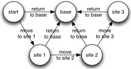
We use a Mars rover domain (Figure 1) that is similar to one used in [Bresina et al., 2002] as an example of our planning problems. A rover has to maximize its expected total reward with time-to-deadline Δ = 4. The states of the MDP correspond to the locations of the rover: its start location, site 1, site 2, site 3 and its base station. The rover can perform two actions with deterministic action outcomes outside of its base station: (1) It can move to the next site and collect a rock probe from there. It receives rewards 4, 2 and 1 for collecting rock probes from sites 1, 2 and 3, respectively. (2) It can also move back to its base station to perform a communication task, which drains its energy completely and thus makes it impossible for the rover to perform additional actions. It receives reward 6 for performing the communication task. All action durations are characterized by the exponential distribution ps,a(t′ ) = e-t′ = E(1). We also consider the case where all action durations are characterized by either Weibull or Normal distributions. The Mars rover domain might appear small with only 5 discrete states. However, if one discretizes the time-to-deadline into 1/100 time units and encodes it in the states, then there are already 5 ∗ 400 = 2000 states.

3 General Approach

We can solve our planning problems by encoding the timeto-deadline in the states, resulting in a continuous state MDP that can be solved with a version of value iteration [Boyan and Littman, 2000] as follows: Let V ∗ (s)(t) denote the largest expected total reward that the agent can obtain until execution stops if it starts in state s ∈ S with time-to-deadline 0 ≤ t ≤ Δ. The agent can maximize its expected total reward by executing the action

in state s ∈ S with time-to-deadline 0 ≤ t ≤ Δ, which can be explained as follows: When it executes action a ∈ A(s) in state s ∈ S, it incurs action duration t′ with probability ps,a(t′ ). If 0 ≤ t′ ≤ t, then it transitions to state s′ ∈ S with probability P (s′ |s, a) and obtains an expected total future reward of R(s, a, s′ ) + V ∗ (s′ )(t - t′ ).

Value iteration calculates the values V n (s)(t) using the following Bellman updates for all states s ∈ S, time-todeadlines 0 ≤ t ≤ Δ, and iterations n ≥ 0

It then holds that limn→∞V n (s)(t) = V ∗ (s)(t) for all states s ∈ S and times-to-deadline 0 ≤ t ≤ Δ. Unfortunately, value iteration cannot be implemented as stated since the number of values V n (s)(t) is infinite for each iteration n since the time-to-deadline t is a real-valued variable. We remedy this situation by viewing the V n (s) as value functions that map times-to-deadline t to the corresponding values V n (s)(t), similar to [Liu and Koenig, 2005]. In this context, we make the following contributions: First, we show after how many iterations n value iteration can stop so that the approximation error maxs∈S,0≤t≤Δ |V ∗ (s)(t)-V n (s)(t)| is no larger than a given constant ϵ > 0. Second, we show that each value function V n (s) can be represented exactly with a vector of a small number of real values each. Finally, we show how the Bellman updates can efficiently transform the vectors of the value functions V n (s) to the vectors of the value functions V n+1 (s). We present these three contributions in the following as three steps of CPH.

4 CPH: Step 1

CPH first approximates the probability distributions of action durations that are not exponential with phase-type distributions, resulting in chains of exponential distributions λe-λt′ = E(λ) with potentially different constants λ > 0 [Neuts, 1981]. CPH then uses uniformization (i.e., creates self-transitions) to make all constants λ identical without changing the underlying stochastic process. We do not give details on how to implement these two well-known steps (see [Neuts, 1981; Younes and Simmons, 2004] for details) but rather provide an example. Figure 2 shows how an action with a deterministic action outcome and an action duration that is characterized by a Normal distribution N (μ = 2, σ = 1) is first approximated with a phase-type distribution with three P=0.03

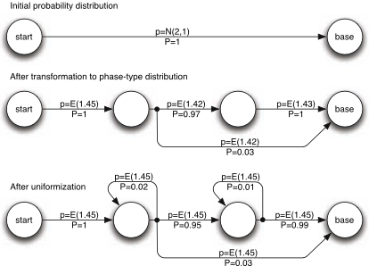
Figure 2: Transformation of a Normal distribution to a chain of exponential distributions E(1.45). p and P denote the action duration and action outcome probabilities, respectively.

phases and then uniformized to yield the exponential distributions E(1.45). From now on, we can therefore assume without loss of generality that the action durations t′ of all actions are distributed according to exponential distributions ps,a(t′ ) = p(t′ ) = E(λ) with the same constant λ > 0. Value iteration cannot determine the value functions V ∗ (s) with a finite number of iterations since the uniformized MDPs have self-transitions. However, Theorem 1 in the appendix shows that the approximation error is no larger than a given constant ϵ > 0 if value iteration stops after at least

iterations, where Rmax :=maxs∈S,a∈A(s),s′∈S R(s, a, s′ ). Running time of Step 1 of CPH is negligible since analytic phase-type approximation methods run in time O(1).

5 CPH: Step 2

It follows directly from the considerations in the next section that there exist times-to-deadline 0 = ts,0 < ts,1 < . . . < ts,ms+1 = Δ such that V n (s)(t) = V n i (s)(t) for all t ∈ [ts,i, ts,i+1), where

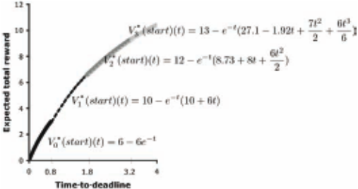
for the parameters cs,i,j for all s ∈ S, 0 ≤ i ≤ ms and 1 ≤ j ≤ n + 1. We refer to the times-to-deadline ts,i as breakpoints, the [ts,i, ts,i+1) as intervals, the expressions for the value functions V n i (s) as gamma functions (which is a simplification since they are actually linear combinations of Euler's incomplete gamma functions), and the expressions for the value functions V n (s) as piecewise gamma functions. We represent each gamma function V n i (s) as a vector [cs,i,1 , . . . , cs,i,n+1] = [cs,i,j ]n+1 j=1 and each piecewise gamma function V n (s) as a vector of vectors [ts,i:V n i (s)]ms i=0 = [ts,i :[cs,i,j ]n+1 j=1 ]ms i=0 . Figure 3, for example, shows the value function V ∗ (start) for our Mars rover domain.

6 CPH: Step 3

We now explain how CPH uses value iteration. For n = 0, the value functions V n (s) = 0 satisfy V n (s) = [0:[0]] and thus are (piecewise) gamma. We show by induction that all value functions V n+1 (s) are piecewise gamma if all value functions V n (s) are piecewise gamma. We also show how the Bellman updates can efficiently transform the vectors of the value functions V n (s) to the vectors of the value functions V n+1 (s). Value iteration calculates

We break this calculation down into four stages: First, V n (s′ )(t - t′ ) := R(s, a, s′ ) + V n (s′ )(t - t′ ). Second, ˜ V n (s′ )(t) := ∫ t 0 p(t′ )V n (s′ )(t - t′ ) dt′ . Third, ̂ V n (s, a)(t) := ∑s′∈S P (s′ |s, a) ˜ V n (s′ )(t). Finally, V n+1 (s)(t) :=maxa∈A(s) ̂ V n (s, a)(t). 1

Stage 1: Calculate V n (s′ )(t - t′ ) := R(s, a, s′ ) + V n (s′ )(t - t′ ). Our induction assumption is that all value functions V n (s′ ) are piecewise gamma, i.e., V n (s′ ) = [ts′ ,i :[cs′ ,i,j ]n+1 j=1 ]ms′ i=0 . In Stage 1, CPH calculates V n (s′ )(t - t′ ) := R(s, a, s′ )+V n (s′ )(t-t′ ), which is the same as calculating V n (s′ )(t) := R(s, a, s′ ) + V n (s′ )(t) since R(s, a, s′ ) is constant. Then,

where c′s′ ,i,1 = R(s, a, s′ ) + cs′ ,i,1 and c′s′ ,i,j = cs′ ,i,j for all 0 ≤ i ≤ms′ and 2 ≤ j ≤ n + 1.

1 We should really use V n (s, a, s′ )(t - t′ ) and e V n (s, a, s′ )(t) instead of V n (s′ )(t-t′ ) and e V n (s′ )(t), respectively, but this would make our notation rather cumbersome.

Stage 2: Calculate ˜ V n (s′ )(t) := ∫ t 0 p(t′ )V n (s′ )(t - t′ ) dt′ , which is a convolution of p and V n (s′ ) denoted as p∗V n (s′ ). Consider the value functions V n (s′ ) defined in Stage 1. We now show by induction that

for all t ∈ [ts′ ,i, ts′ ,i+1). Equation (2) holds for i = 0 since ˜ V n (s′ )(t) = (p ∗ V n0 (s′ ))(t) for all t ∈ [ts′ ,0 , ts′ ,1). Assume now that Equation (2) holds for some i. It then also holds for i + 1 as shown in Figure 4. We use the following lemma to show that ˜ V n i (s′ ) is a gamma function and convert it to vector notation.

Proof. By symbolic integration, p ∗ [k]nj=1 = [k]n+1 j=1 for any constant k. Then, p ∗ [k1 , . . . , kn] = p ∗ (∑n-1 i=1 [ki - ki+1]ij=1 + [kn]nj=1 ) = ∑n-1 i=1 (p ∗ [ki - ki+1]ij=1 )+ p ∗ [kn]nj=1 = ∑n-1 i=1 [ki - ki+1]i+1 j=1 + [kn]n+1 j=1 = [k1 , k1 , . . . , kn].

We now transform Equation (2) to vector notation.

Consequently, ˜ V n (s′ ) = [ts′ ,i:[c′′ s′ ,i,j ]n+2 j=1 ]ms′ i=0 .

̂

Stage 3: Calculate V n (s, a)(t) := ∑s′∈S P (s′ |s, a) ˜ V n (s′ )(t). Consider the value functions ˜ V n (s′ ) defined in Stage 2. Since they might have different breakpoints {ts′ ,i}ms′ i=0 for different states s′ ∈ S with P (s′ |s, a) > 0, CPH introduces the common breakpoints {ts,a,i}ms,a i=0 = ⋃s′∈S:P (s′ |s,a)>0 {ts′ ,i}m′s i=0 without changing the value functions ˜ V n (s′ ). Afterwards, ˜ V n (s′ ) = [ts,a,i:[c′′′ s′ ,i,j ]n+2 j=1 ]ms,a i=0 where c′′′ s′ ,i,j = c′′ s′ ,i′ ,j for the unique i′ with [ts,a,i, ts,a,i+1) ⊆ [ts′ ,i′ , ts′ ,i′+1).

Then,

Stage 4: Calculate V n+1 (s)(t) := maxa∈A(s) ̂ V n (s, a)(t). Consider the value functions ̂ V n (s, a) defined in Stage 3. Since they might have different breakpoints {ts,a,i}ms,a i=0 for different actions a ∈ A(s), CPH introduces common breakpoints ⋃a∈A(s) {ts,a,i}ms,a i=0 without changing the value functions ̂ V n (s, a). CPH then introduces additional dominance breakpoints at the intersections of the value functions to ensure that, over each interval, one of the value functions dominates the other ones. Let {t′s,i }m′s i=0 be the set of breakpoints afterwards. Then, V n+1 (s) = [t′s,i :[c′′′′′ s,i,j ]n+2 j=1 ]m′s i=0 where c′′′′′ s,i,j = c′′′′ s,as,i,i′ ,j for actions as,i ∈ A(s) and the unique i′ with [t′s,i , t′s,i+1 ) ⊆ [ts,as,i,i′ , ts,as,i,i′+1) and, for all t ∈ [t′s,i , t′s,i+1 ), ̂ V n (s, a)(t) ≤ ̂ V n (s, as,i)(t). Furthermore, action as,i should be executed according to the value function V n+1 (s) if the current state is s and the time-todeadline is t ∈ [t′s,i , t′s,i+1 ).

To summarize, the value functions V n+1 (s) are piecewise gamma, and the vectors of the value functions V n (s) can be transformed automatically to the vectors of the value functions V n+1 (s). The lengths of the vectors increase linearly in the number of iterations and, although the number of breakpoints (that are placed automatically during the transformations) can increase exponentially, in practice it stays small since one can merge small intervals after each iteration of value iteration to reduce the number of breakpoints The transformations require only simple vector manipulations and a numerical method that determines the dominance breakpoints approximately, for which CPH uses a bisection method. We now show experimentally that the transformations are both efficient and accurate.

7 Experiments

We performed an experimental feasibility study in our Mars rover domain that compares CPH and Lazy Approximation (LA) [Li and Littman, 2005], currently the leading algorithm for solving continuous state MDPs with quality guarantees (Figure 5). We always plot the error max0≤t≤Δ |V ∗ (start)(t) - V (start)(t)| of the calculated value function V (start) on the x-axis and the corresponding runtime (measured in milliseconds) in log scale on the y-axis.

Experiment 1: We determined how CPH and Lazy Approximation trade off between runtime and error for our Mars rover domain. Since the action durations in the Mars rover domain are already distributed exponentially and thus phasetype with one phase, there are no errors introduced by approximating the probability distributions over the action durations with phase-type distributions. Also, since these distributions are equal, uniformization will not introduce self-transitions and value iteration can run for a finite number of iterations. We therefore varied for CPH the accuracy of the bisection method that determines the dominance breakpoints and for Lazy Approximation the accuracy of the piecewise constant approximations of the probability distributions over the action durations and value functions. Our results show that CPH is faster than Lazy Approximation with the same error, by three orders of magnitude for small errors. For example, CPH needed 2ms and Lazy Approximation needed 1000ms to compute a policy that is less than 1% off optimal, which corresponds to an error of 0.13 in the Mars rover domain.

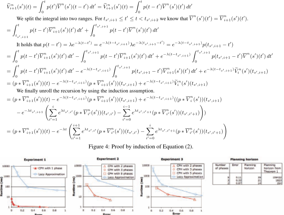
Experiments 2 and 3: We then determined how CPH and Lazy Approximation trade off between runtime and error when all action durations in our Mars rover domain are characterized by either Weibull distributions Weibull(α = 1, β = 2) (Experiment 2) or Normal distributions N (μ = 2, σ = 1) (Experiment 3), and both methods thus need to approximate the value functions. We fixed for CPH the accuracy of the bisection method but varied the the number of phases used to approximate the probability distributions. Our results show that CPH is still faster than Lazy Approximation with the same error, by more than one order of magnitude for small errors. For example, CPH needed 149ms (with five phases) and Lazy Approximation needed 4471ms to compute a policy that is less than 1% off optimal for the Weibull distributions. In addition, we observed that CPH converged much faster than the theoretical planning horizon calculated from Theorem 1 suggests.

8 Conclusions

Planning with real-valued and limited resources can be modeled with continuous state MDPs. Despite recent advances in solving continuous state MDPs, state-of-the art solution methods are still either inefficient [Li and Littman, 2005]

or cannot provide guarantees on the quality of the resulting policy [Lagoudakis and Parr, 2003]. In this paper, we presented a solution method, called CPH, that avoids both of these shortcomings. The aim of this paper was to establish a sound theoretical framework for CPH and provide a first experimental feasibility study to demonstrate its potential. It is future work to study the theoretical properties of CPH in more depth (for example, analyze its complexity or extend its error analysis), evaluate CPH and its three approximations more thoroughly (for example, in larger domains, additional domains and against additional solution methods) and extend CPH (for example, to handle more than one resource, handle replenishable resources or, similarly to Lazy Approximation, approximate its value functions to be able to reduce its number of breakpoints).