Hierarchical Heuristic Forward Search in Stochastic Domains

1 Hierarchical MDPs

A Markov Decision Process (MDP) [Puterman, 1994] is a four-tuple 〈S,A, T,R〉, where S is a set of states, A is a set of actions, T : S × A × S → [0, 1] is the transition function which specifies for every two states s, s′ ∈ S and action a ∈ A the probability of making a transition from s to s′ when a is executed, and R : S×A×S → R is the reward function. We augment the above description with a concrete initial state sinit ∈ S, obtaining a quintuple 〈S, A, T, R, sinit〉. In this paper, we focus on bounded-horizonMDPs (in which the length of each trajectory is bounded by a finite number) and we use the undiscounted expected reward criterion.

We shall concentrate on factored MDPs which have the form 〈X,A, T,R, sinit〉. Here X is a set of state variables, and A, T,R, sinit are as before. The variables in X induce a state space, consisting of the Cartesian product of their domains. To simplify notations, we assume all variables are boolean, that is, they are fluents. Typically, it is assumed that the transition function T is also described in a compact manner that utilizes the special form of the state space, such as dynamic Bayes net [Dean and Kanazawa, 1993] or probabilistic STRIPS rules [Hanks and McDermott, 1994]. In this paper, we do not commit to a concrete action description language, but we expect it to be variable-based, such as the above methods, as we assume that it is easy to identify the relevant variables with respect to an action a ∈ A. This is the set of variables whose value can change when a is executed, as well as those variables that affect the probability by which these variables change their value and the immediate reward received for executing a.

An hierarchical decompositions of an MDP consists of a set of smaller factored MDPs. In its definition, the notion of a projection of T and R plays a central role. Let X ′ be some subset of the variables in X. The projection of T over X ′ w.r.t. action a ∈ A is well defined if a does not affect the value of the variables in X\X ′ and the transition probabilities and reward of a do not depend on the value of these variables. In that case, the actual projection can be obtained by fixing some arbitrary value to the variables in X \ X ′ .

Formally, we define a hierarchical decomposition of a factored MDP M = 〈X,A, T,R, sinit〉 as a tree of factored MDPs, MH = {M0, . . . ,Mn}, where Mi = 〈Xi,A+i , Ti,Ri, sinit i 〉. Each Mi is just a factored MDP. The only difference is that its set of actions, A+i contains a number of special control actions which signify the passing of control to its parent or one of its children. These actions encode the hierarchy, too. More specifically, Xi ⊆ X; A+i is the union of some subset Ai ⊆ A together with two types of control actions: μj corresponds to passing control to a child process Mj , and Abort signifies the passing of control back to the parent process; Ti is the projection of T over Xi, such that Ti is well-defined; Ri depends on Xi and Ai only; and sinit i is the projection of sinit over Xi. In addition, ⋃i=1,...,n Xi = X, ⋃i=1,...,n Ai = A, Ai ∩ Aj = ∅ for every i ̸= j, and whenever x ∈ Xi ∩Xj then x ∈ Xk for every k such that Mk is on the path betweenMi andMj (which is known as the running intersection property). See [Meuleau et al., 2006] for a more detailed description of this model. A decomposition of M into MH can be obtained automatically by a straightforward extension of the methods described in [Amir and Englehardt, 2003] for deterministic planning domains.

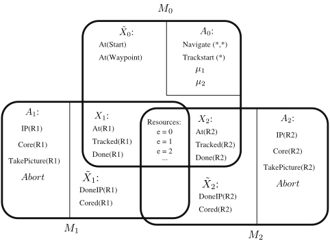
As an illustration, Fig. 1 describes a decomposition of a simple planetary rover domain into three sub-domains. M0 is the top-level domain in which we control the position of the rover and the choice of which subtask to perform next (these are the μi actions). M1 andM2 represent the subtasks associated with experimenting on of one of two rocks. M0 shares some variables with its children, and the resource level is a variable shared by all.

2 Hierarchical AO*

We start with a short review of the AO* algorithm. Next, we show how a hierarchical partition of the search nodes may be exploited to accelerate the algorithm, and we provide the pseudo-code of a new general algorithm called HierarchicalAO* (HiAO*).

• 1: Initialize the explicit graph G to the start state sinit .
• 2: Mark sinit as open.
• 3: while the greedy solution graph contains some open nodes do
• 4: s := any open node of the greedy graph.
• 5: Unmark s as open.
• 6: EXPAND(s). // Expand the greedy graph
• 7: UPDATE(s). // Update state values and mark best actions
• 8: Return the greedy solution graph.

Algorithm 1: Standard AO*.

2.1 The AO* Algorithm

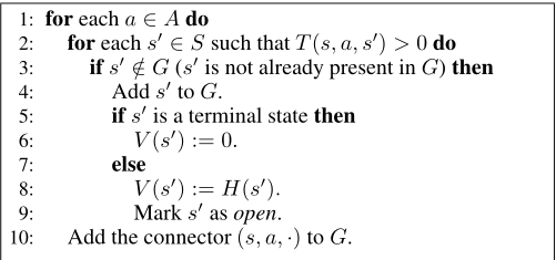
AO* [Nilsson, 1980] is a generalization of A* to And-Or graphs. As such, it can be applied to the problem of generating a policy for an MDP given an initial state, assuming there are no loops in the transition graph [Hansen and Zilberstein, 2001]. In MDPs, an OR node corresponds to a choice of an action at a state, and an AND node corresponds to the set of possible states resulting from each such choice. The possible AND nodes are annotated by their probability.

AO* maintains two basic structures: the explicit graph and the greedy graph. The explicit graph simply depicts the portion of the search space that has been expanded so far. The greedy graph is a subgraph of the explicit graph which represents those nodes that are reachable by the greedy policy. To obtain the greedy graph, one needs to perform dynamic programming in the explicit graph, propagating values bottomup from the leaf nodes (using their heuristic values) to the root node. The value of an AND node is the expected value of its children, and the value of an OR node is the maximum over the value of its children. If we note the choice that yielded this maximum, we can now generate the greedy graph by simply following these choices starting at the root node. The pseudocode for AO* is described in Algorithms 1 - 3.

If an admissible heuristic function is used in AO*, then the value of each node may only decrease at each iteration. 2 When we update the value of a node outside the greedy graph, the greedy graph may not be affected because the update can only reduce the value of the node. Thus, a choice that was sub-optimal cannot become optimal. Consequently, new node values need only be propagated up edges marked as optimal,

2 In a reward-maximization framework, an admissible heuristic is an heuristic that never underestimates the value of a state.

• 1: Create set Z containing only the state s.

2: repeat

• 3: Remove from Z a state s′ such that no descendent of s′ in G occurs in Z.
• 4: Set V (s′ ) :=maxa∈A
• [∑s′′ ∈G T (s′ , a, s′′ ) (R(s′ , a, s′′ ) + V (s′′ ))] and mark the connector associated with the best action in s′ as optimal.
• 5: if V (s′ ) decreased at previous step (it cannot increase) then
• 6: Add all parents of s′ along connectors marked as optimal to Z.
• 7: until Z is empty.

Algorithm 3: UPDATE(s).

• 1: Initialize the explicit graph G to the start state sinit .
• 2: Mark sinit as open.
• 3: SOLVE(S0, sinit ).
• 4: Return the greedy solution graph starting at sinit .

Algorithm 4: Hierarchical AO*.

i.e., denoting the optimal choice in that state.

In most cases, the most expensive parts of AO* are: (1) the update stage, where we propagate value changes up the explicit graph (Alg. 3); (2) the computation of the fringe, that is, the set of open nodes in the greedy graph (line 2 of Alg. 1). We show below how a partition of the states expanded by AO* may be exploited to accelerate these two operations.

2.2 The HiAO* Algorithm

We now assume that the state space S is partitioned into subsets S0, . . . , Sk. Furthermore, we assume that these subsets are organized in a hierarchy in the form of a tree, 3 so that: (1) the starting state sinit belongs to the root subset denoted S0; (2) state transitions are possible only between states in the same subsets, or between two states belonging to two subsets one being the parent of the other. These choices are motivated by the hierarchical MDP framework presented above, where a child subset represents a subprocess that can be called from the current subset/process (therefore, we sometime use the term "subprocess" to designate a child subset). However, our formalism is general and can be applied to any instantiation of AO* where a hierarchy of nodes can be defined.

The HiAO* algorithm is presented in Alg. 4 - 6. The algorithm also uses the same function EXPAND() as standard AO* (Alg. 2). The basic principle of this algorithm is the following: each time that the optimal action in a state leads to a child subset (in other words, each time it appears optimal to call a subprocess from the current state), we recursively call the HiAO* algorithm to solve this child subset completely before continuing solution of the current level. We explain below how this simple mechanism may benefit the algorithm.

3 The algorithm can be generalized to handle hierarchies represented by a directed acyclic graph.

• 1: while the greedy solution graph starting at s contains some open nodes in Si do
• 2: s′ := any open node of the greedy graph starting at s in Si.
• 3: Unmark s′ as open.
• 4: EXPAND(s′ ).
• 5: Mark all nodes created at previous step and that belong to a child of Si as outdated.
• 6: HIERARCHICALUPDATE(Si, s′ ).

Algorithm 5: Function SOLVE(Si, s).

Delaying the propagation of new values: The main principle implemented by HiAO* is to delay the propagation of new node values in between states belonging to different subsets. Let us first consider why delaying updates might be useful. Suppose that we have expanded node u and then node v, and following their expansion, their value has changed. In standard AO*, following the change in value in u we would propagate this information upwards along marked edges. Then, we would repeat the process for v. However, it is quite possible that u and v have common ancestors, and thus we will update these ancestors twice. Sometimes, such an update is important because it influences our choice of which node to expand. Sometimes, such an update can be delayed, and we can save the repeated update of shared ancestors. HiAO* tries to exploit the second case, assuming it happens more often than the first case.

The general scheme we propose for delaying updates is as follows. We associate to each subset Si a set of nodes to update Zi similar to the set Z used in Alg. 3. At any particular point, the algorithm has a single subset of nodes in focus and performs the standard AO* operations only inside of that subset. Whenever a state s ∈ Si is expanded and thus needs to be evaluated, we insert it into Zi and enter a loop that will propagate its value up into the graph by emptying and re-filling the set Zi, as in standard AO* (Alg. 3). However, each time that a new value needs to be propagated to a state s′ belonging to another subset Sj , j ̸= i (Sj is necessarily the parent or a child of Si), s′ is added to Zj and not to Zi (line 18 of Alg. 6), and so, it is excluded from the loop that works only with Zi. So, the propagation is limited to the subset Si, and nodes that would need to be updated but belong to another subset Sj are just stored in Zj, but they are not re-evaluated yet and their new value is not propagated yet.

So, when are the nodes in Sj, j ̸= i updated? The answer depends on the hierarchical relation between Sj on Si. If Sj is the parent of Si, then the states that have been put in Zj during the solution of Si are updated when the algorithm moves focus from Si back to its parent subset Sj. If Sj is child of Si, then the states in Zj are updated at the latest possible time, that is, when we want to evaluate a state outside of Sj that may lead into Sj under the optimal action. This may never happen if calling subprocess Sj is the optimal decision in none of the states visited by the algorithm later on, in which case we save all the work of updating states in Sj. In practice, this is implemented through the use of outdated markers, as explained below.

One of the basic principle of the HiAO* algorithm is that,

• 1: Zi := Zi ∪ {s}.
• 2: while Zi ̸= ∅ do 3: Remove from Zi a state s′ such that no descendent of s′ in G occurs in Zi. 4: Set V (s′ ) :=maxa∈A [∑s′′ ∈G T (s′ , a, s′′ ) (R(s′ , a, s′′ ) + V (s′′ ))], call a∗ (s′ ) the optimal action in s′ , and mark the associated connector as optimal. 5: while executing a∗ (s′ ) in s′ may lead to states that are not in Si and that are marked as outdated do 6: for each child Sj of Si do 7: for each s′′ ∈ Sj such that T(s′ , a∗ (s′ ), s′′ ) > 0 and s′′ is marked as outdated do 8: Unmark s′′ as outdated. 9: HIERARCHICALUPDATE(Sj , NULL). 10: SOLVE(Sj , s′′ ). 11: Set V (s′ ) :=maxa∈A [∑s′′ ∈G T (s′ , a, s′′ ) (R(s′ , a, s′′ ) + V (s′′ ))], call a∗ (s′ ) the optimal action in s′ , and mark the associated connector as optimal. 12: if V (s′ ) decreased at previous step (it cannot increase) then 13: for each state s′′ that is a parent of s′ along a connector marked as optimal do 14: if s′′ ∈ Si then 15: Add s′′ to Zi. 16: else 17: Call Sj , j ̸= i, the subset containing s′′ . 18: Add s′′ to Zj. 19: if Sj is a child of Si then Mark s′′ , and all its predecessors in Sj along
• 20: connectors marked as optimal, as outdated.

Algorithm 6: Function HIERARCHICALUPDATE(Si, s).

when we are done updating a node in Si that can possibly lead to a node s in a child subset Sj (j ̸= i) under the optimal action, then we must know with accuracy the set of optimal decisions that leads from s either to terminal states, or back into Si. A node of Sj is marked as outdated if the greedy subgraph starting at that node has a chance of not being accurate or complete. Suppose that the algorithm is currently working in subset Si and needs to propagate a new value to a state s belonging to a child Sj of Si. Then, as explained above, the update of s is delayed and s is just added to Zj (line 18 of Alg. 6). In addition, all nodes of Sj "above" s in the greedy graph are marked as outdated (line 19 and 20 of Alg. 6). Later, if we want to evaluate a node outside of Sj that can lead to a state s′ ∈ Sj , the value of s′ may not be accurate, because we have delayed propagation of new values in Sj . If this is the case, then s′ must be marked as outdated and, consequently, two operations are performed: (1) we purge the set Zj and update all the nodes in Sj that need to be re-evaluated using a recursive call to HIERARCHICALUPDATE() (line 9 of Alg. 6). This may change the greedy policy in Sj below some of the entry nodes of Sj , including node s′ ; (2) the greedy graph starting at s′ in Sj is updated through a call to SOLVE() (line 10 of Alg. 6). So, the outdated marker in s′ may be deleted (line 8 of Alg. 6), but the markers of all other entry nodes are kept. 4 If we later get to update another state outside of Sj and that can lead to s′′ ∈ Sj, then the outdated marker of s′′ will indicate that the greedy graph below s′′ in Sj needs to be updated, even if no new node has been added to Zj in the mean time.

Convergence: As long as the problemcontains no loop, Hierarchical AO* is guaranteed to terminate in finite time and to return the optimal solution:

Theorem 1 If the heuristic H is admissible, then HiAO* returns the optimal policy in finite time.

HiAO* may not always be efficient, particularly if the number of connections between subsets is large. However, we claim that, in the case of oversubscription planning, the state partition induced by the hierarchy is efficient and allows leveraging the general principle presented above. The simulation results presented in this paper support this claim.

We now present two acceleration techniques that can be implemented in HiAO* to get further leverage from the hierarchy, but are not used in the pseudo-code of Alg. 4 - 6.

Optimizing the algorithm: The HiAO* algorithm presented above exhibits the following inefficiency. If an action a leading to a state s′ ∈ Sj appears optimal in state s ∈ Si (i ̸= j), then the algorithm will SOLVE completely the sub-problem Sj starting in s′ before returning to state s. In the process of solving Sj , the Q-value of action a in s may only decrease, so that it may happen that, before we are done solving Sj, a does not appear as optimal in s anymore. The algorithm presented above will not detect this and singlemindedly continue solving Sj until the greedy policy starting in s′ is known, which can be highly inefficient.

This issue can easily be addressed under an additional hypothesis that is satisfied in the hierarchical planning context described above and that could easily be relaxed to deal with a more general case. We assume that each action either does not change the partition subset (in the case of hierarchical planning, this holds true for all primitive actions a ∈ A), or it leads with certainty to a single state belonging to a different subset (this is the case of control passing actions μi and Abort). Then, we can modify the algorithm by adding a threshold parameter τ to the function SOLVE(S, s) so that, when the value of s falls below τ during the solution of S, the function exits. In the initial call to SOLVE (line 3 of Alg. 4), the threshold parameter is set to -∞, so that optimization will be pursued until its end. Later calls (line 10 of Alg. 6) are performed in the following way: while computing the value of a state (lines 4 and 11 of Alg. 6), we record the Q-value of the best action that does not change the partition subset (primitive action), the Q-value of the best action that induce a change of subset (control-passing action), and the Q-value of the second best control-passing action. If a control-passing action appears optimal and we enter the loop in lines 5 to 11, then the threshold parameter τ used for the call to SOLVE() in line 10 is set to the Q-value of the best primitive action, or the second best control-passing action, depending on which is greater. In this way, SOLVE aborts the solution of a child subset as soon as the action leading into it does not appear optimal anymore. Note that the outdated marker is removed (line 8 of Alg. 6) only if SOLVE completed.

4 A straightforward improvement to the algorithm is to delete the outdated marker in all nodes of Sj belonging to the greedy graph starting in s′ after recomputing this graph.

By-passing levels: Two of the operations of standard AO* require it to traverse up or down a large part of the explicit graph. The function EXPAND() selects a node on the fringe of the greedy graph. This requires computing the fringe, which is done by following marked edges down from the root note. This operation is often one of the most costly. 5 The function UPDATE() also propagates information up the graph, when determining the greedy parents of a recently updated nodes (line 6 of Alg. 3). Because HiAO* performs the standard AO* operations only inside of a subset of nodes, it saves time on both operations. First, the search graph projected to each subset is smaller, so that the size of the fringe for that subset and the time to compute it is likely to be (much) smaller. Of course, by doing this, we expand the most promising fringe node in a given subset, and not in the entire greedy graph as AO* does. So, we influence the order in which nodes are selected for expansion, which may have good or bad consequences. Second, as explained before, HiAO* postpones the propagation of some values from a subset to another other, and thus limits the propagation of information up in the graph.

To gain more leverage, HiAO* may be augmented with macro-connectors that represent the effect of applying the greedy solution for a subset of nodes. Macro-connectors are then used when solving other subsets, to accelerate the traverse of the graph. Imagine, for instance, that u belongs to Si, and applying some action a leads from u to u′ ∈ Sj, j ̸= i, and then applying a′ leads from u′ to u′′ ∈ Si. Then, we add an explicit edge between u and u′′ and we use it when solving Si. By doing this, we build, in effect, a projection of the greedy graph on Si. The new edge between u and u′′ helps us during the solution of Si in two circumstances: when we compute the fringe, we can jump over a large number of states that flat AO* would have considered individually; and similarly when we determine the greedy parents of a recently updated node. Creating and maintaining macro-connectors increases the complexity of HiAO* slightly, but the efficiency gained compensates for this extra cost. Indeed, our simulations showed that this is one of the major causes of the good performances exhibited by our algorithm.

3 Application to Oversubscription Planning

We now focus on the class of problems that motivates this work, that is, oversubscribed planning problems. Following [Meuleau et al., 2006], these problems are naturally modelled in the hierarchical planning framework presented above with a two-level hierarchy. There is a single root process M0

5 It is possible to store the fringe and update it as we progress, but it turns out that because the structure we are searching is a directed acyclic graph, not a tree, this is a costly operation.

and multiple leaf/child processes Mi, i = 1, . . . n representing the different subtasks the agent can select to perform. For each subprocess Mi, we define:

• ¯Xi = Xi ∩X0 are the separator (shared) variables between M0 and Mi. The shared variables include, but are not limited to, the shared resource levels. They may also include, for instance, the state of instruments used to perform several subtasks.
• ˜Xi = Xi \X0 are the private variables of Mi. Typically, they represent the state of advancement of the subtask.
• X0-i =X0 \Xi is the difference of M0 andMi.

The set of private variables of M0 is defined as ˜X0 = X0 \ ⋃ni=1 Xi = ⋂ni=1 X0-i. We also define various classes of states: S = 2X , Si = 2Xi , ¯ Si = 2 ¯Xi , ˜ Si = 2 eXi , S0-i = 2X0-i .

We restrict our attention to domain satisfying the reset assumption of [Meuleau et al., 2006]. The reset assumption states that whenever the process moves into a child sub-MDP, the state of the private variables of this sub-MDP is the same. It holds true in the rover domain because the rover must have its arm stowed and all of its instruments parked prior to any movement, and so, this is its configuration when it arrives at a new rock/subtask. Moreover, actions of preparing the rock for a measurement, such as coring the rock, have to be redone if we abort this rock before completing the measure, because it is not possible to put the rover arm exactly at the place it was when the rock was cored. So, all intermediate work towards the goal is lost once we move to another rock. Note that variables that are not private to the child sub-MDP, such as resource levels, are not reset to their initial value when we abort the subtask. Note also that this assumption is not as restrictive as it may look, since the user may modify the sets ¯XI if needed: if some intermediate work may be preserved when we abort a subtask Mi before its completion, then the fluent representing this intermediate state should be moved from ˜Xi to ¯Xi. However, HiAO*, as well as the algorithms in [Meuleau et al., 2006], work better if the separation sets are as small as possible.

Under the reset assumption, the space of reachable states is naturally partitioned into a hierarchy of subsets. The root subset S0 represents the states where all subtasks are in their initial condition. For each subtask i and each state s0-i ∈ S0-i, there is a child subset Si[s0-i] containing all states where (1) Mi is not in its initial condition, (2) the private variable of every other subtasks Mj, j ̸= i, have their initial value, and (3) the variables in X0-i are equal to s0-i, and so, s0-i represents the context in which subtask i is called. All other states, for instance, states where two subtask are not in their initial state, are not reachable. The Abort-Update algorithm of [Meuleau et al., 2006] is an instance of Asynchronous Policy Iteration [Bertsekas and Tsitsiklis, 1997] that that exploits this property. Here, we stress that this hierarchical partition may serve as the basis to an implementation of HiAO*. In a sense, HiAO* is to Abort-Update what standard AO* is to Policy Iteration.

Reusing macro-actions: As explained above, when we apply HiAO* on an oversubscribed planning problem, there is a subset Si[s0-i], for each subtaskMi and each context s0-i in which Mi may be started. For a fixed i, the dynamics within Si[s0-i] do not depend on the context s0-i. The latter influences the value of states where we transit when we abort the subtask (the exit values), and so, the optimal policy, but not the structure of the explicit graph representing Si[s0-i]. Therefore, if we have computed part of the explicit graph for a given context, we can reuse/copy it when we want to solve the same subtask in another context. We might need to expand this graph further, because different exit values may induce different policies. Similarly, this seed may contain some nodes that we would not have created if we started the solution of subtask i in the new context from scratch. However, we could benefit from this because much of the work of expanding the graph is already done.

Optimality: HiAO* finds the optimal solution within the predefined hierarchy, which is the definition of hierarchical optimality[Andre and Russell, 2002]. As shown in [Meuleau et al., 2006], if the problem satisfies the reset assumption, then there is an absolute optimal policy that can be encoded in the hierarchy defined above. Therefore, HiAO* finds the optimal policy if the reset assumption holds. If the reset assumption does not hold, HiAO* based on the hierarchy defined above finds an hierarchical optimal policy, which may be of lesser value than an absolute optimal policy. However, we can use a different hierarchical representation of the problem that would guarantee absolute optimality. This is achieved by defining a subset Si[s-i] for each subtask Mi and each state s-i ∈ S-i = 2X\Xi (note that, now, the context also includes the private variable of subtasks Mj , for all j ̸= i).

4 Experimental Evaluation

The goal of our empirical evaluation is to show that the fundamental structural changes of HiAO* are beneficial. For this purpose, we used several problem instances from a complex planetary rover domain. In this domain, an autonomous rover must navigate in a discrete graph representing its surrounding and the authorized navigation paths, and schedule observations to be performed on different rocks situated at different locations. Each action as an uncertain positive resource consumption and a probability of failing. The domain also contains a significant amount of uncertainty coming from the tracking mechanism: To perform some measurement on a rock, the rover must be tracking this rock; and to navigate along a path, it must be tracking one of the rocks that enables following this path. However, the rover may randomly loose track of some rocks while navigating along some path, and there is no way to re-acquire a rock once the rover lost track of it (the probability of losing track of a rock depends on the rock and the path followed). Each problem instance is naturally decomposed in a two-level hierarchy where the root task is responsible for navigating in the graph, tracking the rocks, and performing some measures that are not bound to a rock, such as taking a panoramic camera picture. Each subtask represent a rock and may possibly contain several goals (several measures may be taken on the rock).

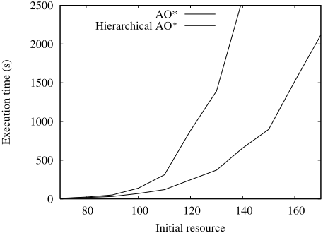
Our test problems are far out of reach of standard flat MDP solvers such as Value Iteration, as well as hierarchical algorithms based on flat MDP solvers such as the Abort-Update algorithm of [Meuleau et al., 2006]. For instance, the problem used in Fig. 2, with an initial resource of 100, as a total number of 71 fluents, and so 271 states, which is way above what a standard MDP solver can handle. Once the problem is hierarchically decomposed, the root MDP contains 53 fluents (and so, 253 states), and each sub-MDP contains 39 fluents (239 states), and so, it cannot be solved by AbortUpdate. Therefore, HiAO* outperforms approaches based on flat MDP solvers. This is due to the well-known advantage of reachability and heuristic information that focus the search only on the relevant parts of the state space.

It is more interesting is to compare HiAO* with standard AO*, which uses reachability and heuristic information, but does not leverage from the hierarchical structure of the domain. Figure 2 presents a typical performance curve. It was obtained using a problem instance involving 3 rocks, 2 goals per rock, and 2 goals in the root process (panoramic images). It shows the evolution of the solution time of standard AO* and HiAO* as a function of the initial resource available to the rover. Although the complexity of the problem increases badly with the initial resource, this increase is much less in HiAO* due to the savings during value updates and graph traversal. Very similar results were obtained with nearly all problem instances that we tried, the advantage of HiAO* increasing with the problem size. The only exceptions are tiny problem instances that are solved in fraction of seconds by both algorithms.

The results depicted above were obtained using a version of HiAO* that implements delayed propagation, as described above, and that uses macro-connectors to by-pass subprocess states when solving the root process. These two principles are pretty general and can be implemented in any instance of AO*, provided that a hierarchical partition of the state space is defined. However, the algorithm used does not implement macro-action re-use, which is more specific to oversubscription planning. We tried macro-action re-use but did not observe any significant change in the solution time with this option turned on (we sometimes observed a very small decrease in the performances). In a sense, this is pretty encouraging, as the most general modifications to standard AO* search turn out to be also the most efficient.

5 Conclusions

We showed how AO* can be modified to make use of hierarchical decompositions of a domain. This leads to the first forward search algorithm that explicitly deals with hierarchical domains. We analyzed the relationship between standard AO* and the hierarchical version in terms of its effect on the order of propagation and the introduction of shortcuts in the form of edges that by-pass levels. Although there is no formal guarantee that these modifications will induce an actual performance improvement, our experimental evaluation using over-subscribed planning problems indicate that they are, indeed, beneficial. Therefore, this paper outlines research directions that could benefit a wide variety of application domains, and possibly other forward search algorithms. In future work, we shall examine an additional possible benefit of hierarchical decompositions: the ability to formulate specialized and more accurate heuristic functions.

Acknowledgements

This work was supported by NASA Intelligent Systems program under grant NRA2-38169. This work was performed while Ronen Brafman was visiting NASA Ames Research Center as a consultant for the Research Institute for Advanced Computer Science. Ronen Brafman was supported in part by The Paul Ivanier Center for Robotics Research and Production Management and the Lynn and William Frankel center for Computer Sciences at Ben-Gurion University.