
Limited Discrepancy Beam Search
Proceedings of the Nineteenth International Joint Conference on Artificial Intelligence. Pages 125-130.
© 2005 International Joint Conferences on Artificial Intelligence
Abstract
Beam search reduces the memory consumption of bestfirst search at the cost of finding longer paths but its memory consumption can still exceed the given memory capacity quickly. We therefore develop BULB (Beam search Using Limited discrepancy Backtracking), a complete memory-bounded search method that is able to solve more problem instances of large search problems than beam search and does so with a reasonable runtime. At the same time, BULB tends to find shorter paths than beam search because it is able to use larger beam widths without running out of memory. We demonstrate these properties of BULB experimentally for three standard benchmark domains.
- [Bisiani, 1987] R. Bisiani. Beam search. In S. Shapiro, editor, En- cyclopedia of Artificial Intelligence, pages 56-58. Wiley & Sons, 1987.
- [Chakrabarti et al., 1989] P. Chakrabarti, S. Ghose, A. Acharya, and S. de Sarkar. Heuristic search in restricted memory. Arti- ficial Intelligence, 41(2):197-221, December 1989.
- [Chu and Wah, 1992] L.-C. Chu and B. Wah. Band search: An ef- ficient alternative to guided best-first search. In Proceedings of the International Conference on Tools for Artificial Intelligence, pages 154-161. IEEE Computer Society Press, November 1992.
- [Felner et al., 2003] A. Felner, S. Kraus, and R. Korf. KBFS: K- best-first search. Annals of Mathematics and Artificial Intelli- gence, 39:19-39, 2003.
- [Felner et al., 2004] A. Felner, R. Meshulam, R. Holte, and R. Korf. Compressing pattern databases. In Proceedings of the National Conference on Artificial Intelligence, pages 638-643, 2004.
- [Furcy and Koenig, 2005] D. Furcy and S. Koenig. Scaling up WA* with commitment and diversity. In Proceedings of the Interna- tional Joint Conference on Artificial Intelligence, 2005. IJCAI
- [Furcy, 2004] D. Furcy. Speeding up the Convergence of Online Heuristic Search and Scaling Up Offline Heuristic Search. PhD thesis, College of Computing, Georgia Institute of Technology, Atlanta (Georgia), 2004. Available as Technical Report GIT- COGSCI-2004/04.
- [Hansen et al., 1997] E. Hansen, S. Zilberstein, and V. Danilchenko. Anytime heuristic search: First results. Technical Report CMPSCI 97-50, Department of Computer Science, University of Massachusetts, Amherst (Massachusetts), 1997.
- [Harvey and Ginsberg, 1995] W. Harvey and M. Ginsberg. Lim- ited discrepancy search. In Proceedings of the International Joint Conference on Artificial Intelligence, pages 607-615, 1995. IJCAI
- [Hernádvölgyi, 2001] I. Hernádvölgyi. Searching for macro oper- ators with automatically generated heuristics. In Proceedings of the Canadian Conference on Artificial Intelligence, pages 194- 203, 2001.
- [Kaindl and Khorsand, 1994] H. Kaindl and A. Khorsand. Memory-bounded bidirectional search. In Proceedings of the National Conference on Artificial Intelligence, pages 1359-1364, 1994.
- [Kitamura et al., 1998] Y. Kitamura, M. Yokoo, T. Miyaji, and S. Tatsumi. Multi-state commitment search. In Proceedings of the International Conference on Tools for Artificial Intelligence, pages 431-439, 1998.
- [Korf and Taylor, 1996] R. Korf and L. Taylor. Finding optimal so- lutions to the twenty-four puzzle. In Proceedings of the National Conference on Artificial Intelligence, pages 1202-1207, 1996.
- [Korf, 1990] R. Korf. Real-time heuristic search. Artificial Intelli- gence, 42(2-3):189-211, 1990.
- [Korf, 1993] R. Korf. Linear-space best-first search. Artificial In- telligence, 62(1):41-78, 1993.
- [Korf, 1997] R. Korf. Finding optimal solutions to Rubik's cube us- ing pattern databases. In Proceedings of the National Conference on Artificial Intelligence, pages 700-705, 1997.
- [Pearl, 1985] J. Pearl. Heuristics: Intelligent Search Strategies for Computer Problem Solving. Addison-Wesley, 1985.
- [Russell, 1992] S. Russell. Efficient memory-bounded search meth- ods. In Proceedings of the European Conference on Artificial Intelligence, pages 1-5, 1992.
- [Shell et al., 1994] P. Shell, J. Rubio, and G. Barro. Improving search through diversity. In Proceedings of the National Con- ference on Artificial Intelligence, pages 1323-1328, 1994.
- [Walsh, 1997] T. Walsh. Depth-bounded discrepancy search. In Proceedings of the International Joint Conference on Artificial Intelligence, pages 1388-1393, 1997. IJCAI
- [Zhang, 1998] W. Zhang. Complete anytime beam search. In Pro- ceedings of the National Conference on Artificial Intelligence, pages 425-430, 1998.
- [Zhou and Hansen, 2002] R. Zhou and E. Hansen. Memory- bounded A* graph search. In International FLAIRS Conference, 2002.
- [Zhou and Hansen, 2004] R. Zhou and E. Hansen. Breadth-first heuristic search. In Proceedings of the International Conference on Automated Planning and Scheduling, pages 92-100, 2004.
References were extracted automatically from the PDF and may contain errors.
Full text extracted automatically from the PDF; figures, tables and equations may differ. The PDF is the version of record.
1 Introduction
Best-�rst search methods, such as A*, do not scale up to large search problems due to their memory consumption, and linear-space best �rst search methods [Korf, 1993] have unacceptable runtimes for large search problems. Beam search reduces the memory consumption of best-�rst search at the cost of �nding longer paths. It uses breadth-�rst search to build its search tree but keeps at most the B states at each level of the search tree with the smallest heuristic values, where the value of the beam width B is set at the beginning of the search. The smaller the beam width, the more states beam search prunes at each step of the search and the less memory it needs to store each level of the search tree. Unfortunately, more pruning typically increases the probability of pruning states on short paths from the start state to a goal state and thus often increases the lengths of the paths found. Excessive pruning can even prevent one from �nding any path. Thus, the beam width has to be large. Our experiments show, for example, that beam search with a beam width of 10,000 solves about eighty percent of random problem instances of the 48-Puzzle. The average path length found is on average about one order of magnitude smaller than the one found by variants of WA* [Pearl, 1985], which are alternatives to beam search that also
∗The Intelligent Decision-Making Group is partly supported by NSF awards to Sven Koenig under contracts IIS-0098807 and IIS0350584. The views and conclusions contained in this document are those of the authors and should not be interpreted as representing the of�cial policies, either expressed or implied, of the sponsoring organizations, agencies, companies or the U.S. government.
Sven Koenig
University of Southern California Computer Science Department Los Angeles, CA 90089-0781 skoenig@usc.edu
reduce the memory consumption of best-�rst search at the cost of �nding longer paths. We develop BULB (Beam search Using Limited discrepancy Backtracking) that is able to solve more problem instances of large search problems than beam search, and does so with a reasonable runtime. At the same time, BULB tends to �nd shorter paths than beam search because it is able to use larger beamwidths without running out of memory. It behaves like beam search until it exhausts the memory capacity without �nding a path. It then uses limited discrepancy backtracking to retract its previous pruning decisions. The choice of a good backtracking strategy is important since, for example, beam search with chronological backtracking has unacceptable runtimes.
2 Beam Search
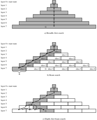
Beam search is any search technique �in which a number of [...] alternatives (the beam) are examined in parallel. [It] is a heuristic technique because heuristic rules are used to discard [prune] non-promising alternatives in order to keep the size of the beam as small as possible� [Bisiani, 1987]. We assume that all actions have a cost of one and study beam-search variants of breadth-�rst search in this paper. Their objective is to reduce the memory consumption of breadth-�rst search from exponential to linear in the depth of the search tree, as illustrated by the shaded areas of Figure 1 (a) and (b) for breadth�rst search and beam search, respectively. Beam search uses breadth-�rst search to build its search tree but splits each level of the search tree into slices of at most B states, where B is called the beam width. The number of slices stored in memory is limited to one at each level. When beam search expands a level, it generates all successors of the states at the current level, sorts them in order of increasing heuristic values (from left to right in the �gure), splits them into slices of at most B states each, and then extends the beam by storing the �rst slice only. Beam search terminates when it generates a goal state or runs out of memory.
| B | Path Length | Generated States | Stored States | Runtime (Seconds) | Problems Solved |
| 1 | N/A | N/A | N/A | N/A | 0 % |
| 5 | 11,737.12 | 147,239 | 58,680 | 0.090 | 100 % |
| 10 | 36,281.64 | 904,632 | 362,799 | 0.601 | 100 % |
| 50 | 25,341.44 | 3,211,244 | 1,266,902 | 2.495 | 86 % |
| 100 | 12,129.88 | 3,079,594 | 1,212,579 | 2.296 | 86 % |
| 500 | 2,302.86 | 2,899,765 | 1,148,559 | 2.205 | 74 % |
| 1,000 | 1,337.95 | 3,346,004 | 1,331,451 | 2.822 | 84 % |
| 5,000 | 481.30 | 5,814,061 | 2,365,603 | 5.500 | 86 % |
| 10,000 | 440.07 | 10,569,816 | 4,312,007 | 11.307 | 80 % |
| 50,000 | N/A | N/A | N/A | N/A | 0 % |
Table 1 shows experimental results for beam search on the 48-Puzzle with a memory limitation of 6,000,000 states. We created 50 problem instances with random start con�gurations in which the goal con�guration had the blank in the upper left corner. We used the Manhattan distance as heuristic function. (We could have used pattern databases instead [Korf and Taylor, 1996] but did not since we use them later in this paper in the context of 2 additional benchmark domains.) The runtime of beam search was always small since it ran out of memory in seconds. Beam search with a beam width of 1 solved none of the problem instances. This is not surprising since it is similar to greedy search (gradient descent) and thus likely to �nd rather long paths unless it gets stuck in dead ends because the current state has only successors that are already in memory, in which case it does not �nd any path at all. Beam search with a beam width of 10 solved all of the problem instances. As the beamwidth increased, its memory consumption increased, the average path length of the solved problem instances decreased, and the number of solved problem instances eventually decreased. Beam search with beam width 50,000 solved none of the problem instances. This is not surprising since beam search with a beam width of in�nity is breadth-�rst search and thus guaranteed to �nd shortest paths unless it runs out of memory and then does not �nd any path at all, which is likely given the exponential memory consumption of breadth-�rst search. Consider beam search with a large beamwidth that still solved a substantial number of problem instances, say beam search with a beam width of 10,000 that solved eighty percent of the problem instances. The average path length of the solved problem instances was an order of magnitude smaller than the one reported in [Furcy,
2004] for several variants of WA*.
3 Improving Beam Search
We study how to increase the number of solved problem instances to one hundred percent while reducing the path lengths of the solved problem instances. This cannot be done by varying the beam width since increasing it reduces the number of solved problem instances while decreasing it increases the average path length of the solved problem instances. Rather, we notice that many of the unsolved problem instances are due to misleading heuristic values that prevent states from being included in the beam. For example, the goal state G is put into the third slice of the seventh layer in Figure 1 (b). Beam search thus does not �nd the goal state since it visits only the �rst slice of each layer. Our solution to this problem is to backtrack and choose a different slice. Figure 1 (c) shows DB (Depth-�rst Beam search), our simplest variant of beam search with backtracking. DB behaves like beam search until it exhausts the memory capacity without �nding a path. It then uses chronological backtracking to purge existing slices and replace them with others. DB, unfortunately, has unacceptable runtimes, which we explain as follows: Chronological backtracking revisits the most recent decisions �rst, that is, the decisions close to the bottomof the search tree. This is problematic since the heuristic values are usually the more inaccurate the farther a state is away from the goal state and thus the closer it is to the top of the search tree. Thus, it is important to revisit decisions close to the top of the search tree more quickly. We therefore use limited discrepancy search rather than chronological backtracking to build a more sophisticated variant of beam search with backtracking.
3.1 Original Limited Discrepancy Search
LDS (Limited Discrepancy Search) [Harvey and Ginsberg, 1995] was designed to work on �nite binary trees. The successors of a state are sorted in order of increasing heuristic values. Thus, the heuristic values always recommend the left successor over the right one. Choosing the right successor against the recommendation of the heuristic values is called a discrepancy. First, LDS searches the tree greedily, that is, with no discrepancy. If LDS does not �nd a goal state, then it made at least one wrong decision due to misleading heuristic values. LDS then searches the tree with increasing numbers of allowed discrepancies. Figure 2 contains the pseudo code of LDS. The top-level function LDS() repeatedly performs a limited discrepancy search from the start state (Line 4) by calling LDSprobe() with an increasing number of allowed discrepancies (Line 6), starting with no discrepancy (Line 2). Unless the current state is a leaf of the tree (Line 9), LDSprobe() generates its successors and recursively calls itself on them. If the maximum number of allowed discrepancies is zero, then only the sub-tree below the best successor is visited with no discrepancy allowed (Line 12). Otherwise, the sub-tree under the worst successor is visited with one less discrepancy allowed (since one was just consumed, Line 14), then the sub-tree under the best successor is visited with the same number of allowed discrepancies (since none was con-
1. procedure LDS(sstart , h(.)): path length 2. discrepancies := 0 3. while ( true ) do 4. cost := LDSprobe(sstart , 0, discrepancies, h(.)) 5. if ( cost < ∞ ) then return cost 6. discrepancies := discrepancies + 1 7. end while 8. procedure LDSprobe(state, depth, discrepancies, h(.)): path length 9. if ( state is a leaf ) then return∞ 10. else 〈best, second〉 := generateSuccessors(state) 11. if ( (best = sgoal ) or (second = sgoal ) ) then return depth + 1 12. if ( discrepancies = 0 ) then return LDSprobe(best, depth + 1, 0, h(.)) 13. else 14. cost := LDSprobe(second, depth +1, discrepancies - 1, h(.)) 15. if ( cost < ∞ ) then return cost 16. return LDSprobe(best , depth + 1, discrepancies , h(.))1. procedure GLDS(sstart , h(.)): pathlength 2. discrepancies := 0; hashtable := {sstart} 3. while ( true ) do 4. pathlength := GLDSprobe(sstart , 0, discrepancies, h(.)) 5. if ( pathlength < ∞ ) then return pathlength 6. discrepancies := discrepancies + 1 7. end while 8. procedure GLDSprobe(state, depth, discrepancies, h(.)): path length 9. SET := ∅ 10. for each successor s of state do 11. if ( s = sgoal ) then return depth + 1 12. if ( s /∈ hashtable ) then SET := SET ∪{s} 13. end for 14. if ( SET = ∅ ) then return∞ 15. if ( hashtable has only one empty slot ) then return∞ 16. best := arg mins∈SET { h(s) } 17. if ( discrepancies = 0 ) then 18. hashtable := hashtable ∪ {best} 19. pathlength := GLDSprobe(best, depth + 1, 0, h(.)) 20. else 21. SET := SET\{best} 22. while ( SET ̸= ∅ ) do 23. state := arg mins∈SET { h(s) } 24. SET := SET\{state} 25. hashtable := hashtable ∪ {state} 26. pathlength := GLDSprobe(state, depth + 1, discrepancies - 1, h(.)) 27. hashtable := hashtable\{state} 28. if ( pathlength < ∞ ) then return pathlength 29. end while 30. hashtable := hashtable ∪ {best} 31. pathlength := LDSprobe(best, depth + 1, discrepancies, h(.)) 32. hashtable := hashtable\{best} 33. return pathlengthsumed at the current level by following the heuristic recommendation, Line 16). LDS terminates when it generates the goal state (Line 11).
3.2 Generalized Limited Discrepancy Search
To apply LDS to beam search, we need to generalize it from binary trees to arbitrary graphs. First, LDS must be able to handle branching factors that are nonuniform and larger than two. Second, LDS must be able to avoid cycles. GLDS (Generalized Limited Discrepancy Search) addresses the �rst issue by picking a successor s of a given state with a smallest heuristic value h(s). Choosing any other successor is counted as one discrepancy, and the successors are tried from left to right. GLDS addresses the second issue by performing cycle detection with a hash table and not generating successors that are already in the hash table. Figure 3 shows the pseudo code for GLDS. The top-level function GLDS() repeatedly performs generalized limited discrepancy searches from the start state (Line 4) by calling GLDSprobe() with an increasing number of allowed discrepancies (Line 6), starting with no discrepancy (Line 2). GLDSprobe() performs a generalized
1. procedure BULB(sstart , h(.), B): path length 2. discrepancies := 0; g(sstart) := 0; hashtable := {sstart} 3. while ( true ) do 4. pathlength := BULBprobe( 0, discrepancies, h(.), B) 5. if ( pathlength < ∞ ) then return pathlength 6. discrepancies := discrepancies + 1 7. end while 8. procedure BULBprobe(depth, discrepancies, h(.), B): path length 9. 〈SLICE, value, index〉 := nextSlice(depth, 0, h(.), B) 10. if ( value ≥ 0 ) then return value 11. if ( discrepancies = 0 ) then 12. if ( SLICE = ∅ ) then return∞ 13. pathlength := BULBprobe(depth +1, 0, h(.), B) 14. for each s in SLICE do hashtable := hashtable\{s} end for 15. return pathlength 16. else 17. if ( SLICE ̸= ∅ ) then 18. for each s in SLICE do hashtable := hashtable\{s} end for 19. while ( true ) do 20. 〈SLICE, value, index〉 := nextSlice(depth, index , h(.), B) 21. if ( value ≥ 0 ) then 22. if ( value < ∞ ) then return value 23. else break 24. if ( SLICE = ∅ ) then continue 25. pathlength := BULBprobe(depth+1, discrepancies -1, h(.), B) 26. for each s in SLICE do hashtable := hashtable\{s} end for 27. if ( pathlength < ∞ ) then return pathlength 28. end while 29. 〈SLICE, value, index〉 := nextSlice(depth, 0, h(.), B) 30. if ( value ≥ 0 ) then return value 31. if ( SLICE = ∅ ) then return∞ 32. pathlength := BULBprobe(depth +1, discrepancies, h(.), B) 33. for each s in SLICE do hashtable := hashtable\{s} end for 34. return pathlength 35. procedure nextSlice(depth,index ,h(.),B): 〈 array of states, integer, integer 〉 36. currentlayer := {s ∈ hashtable | g(s) = depth} 37. SUCCS := generateNewSuccessors(currentlayer, h(.)) 38. if ( (SUCCS = ∅) or (index = |SUCCS|) ) then return 〈∅,∞,-1〉 39. if ( sgoal ∈ SUCCS ) return 〈∅, depth + 1, -1〉 40. SLICE := ∅; i := index 41. while ( (i < |SUCCS|) and (|SLICE| < B) ) do 42. if ( SUCCS[i] /∈ hashtable ) then 43. g(SUCCS[i]) := depth; SLICE := SLICE ∪ {SUCCS[i]} 44. hashtable := hashtable ∪ {SUCCS[i]} 45. if ( hashtable is full ) then 46. for each s in SLICE do hashtable := hashtable\{s} end for 47. return 〈∅, ∞, -1〉 48. i := i + 1 49. end while 50. return 〈SLICE, -1, i〉 51. procedure generateNewSuccessors(stateset, h(.)): array of states 52. index := 0 53. for each state in stateset do 54. for each successor s of state do 55. if ( s /∈ hashtable ) then 56. SUCCS[index] := s; index := index + 1 57. end for 58. end for 59. Sort states in SUCCS in order of increasing h(.)-values 60. return SUCCSlimited discrepancy search from a given state for a given number of allowed discrepancies. First, it generates all successors of the state that are not already in the hash table (Lines 9-13). It backtracks if the goal state is found (Line 11), there are no successors (Line 14), or the hash table is full (Line 15). Otherwise, it identi�es the best successor as one with a smallest heuristic value (Line 16). If the number of allowed discrepancies is zero, then GLDSprobe() calls itself on the best successor with no allowed discrepancies (Line 19). Otherwise, GLDSprobe() calls itself repeatedly on the remaining successors with one less allowed discrepancy (Line 26) and then calls itself on the best successor with the same number of allowed discrepancies (Line 31).
3.3 BULB
BULB (Beam search Using Limited discrepancy Backtracking) combines beam search with GLDS. Figure 4 shows the pseudo code for BULB. The top-level function BULB() is basically identical to GLDS(). The function BULBprobe() performs beam search with generalized limited discrepancy search for a given number of allowed discrepancies. It �rst generates the �rst slice of the next level (Line 9). If the slice contains a goal state, the slice is empty, the subtree has been searched exhaustively, or the hash table (which stores the beam) is full, then it aborts (Lines 10 and 12). If the number of allowed discrepancies is zero (Line 11) and the slice is not empty (Line 12), then BULBProbe() calls itself with no allowed discrepancies (Line 13), and clears the hash table of the slice (Line 14). Otherwise, BULBProbe() clears the hash table of the slice (Line 18), calls itself repeatedly on the remaining slices with one less allowed discrepancy (Line 25) and then calls itself on the best slice with the same number of allowed discrepancies (Line 32). The function nextSlice() generates a successor slice for a slice that is already in the hash table at a given depth. It �rst locates the given slice (Line 36), generates all successors of its states (Line 37), and then locates the slice of the given index within the successors. It does this by inserting successors into both an empty slice (Line 43) and the hash table (Line 44), starting with the successor at the given index (Line 40), until either B successors have been inserted into the slice or the end of the layer has been reached (Line 41). If the hash table is full (Line 45), then it clears the hash table of the incomplete slice (Line 46) and aborts (Line 47). The function generateNewSuccessors() generates the successors s of a given set of states that are not already in the hash table and sorts them in order of increasing heuristic values h(s). (The successors can contain duplicates.)
| beam width | type of backtracking | ||
|---|---|---|---|
| none | chronological | limited discrepancy | |
| 1 | greedy search (gradient descent) | guided depth-�rst search | limited discrepancy search (LDS/GLDS) |
| intermediate values | beam search | depth-�rst beam search (DB) | beam search using limited discrepancy backtracking (BULB) |
| ∞ | breadth-�rst search | breadth-�rst search | breadth-�rst search |
3.4 Properties of BULB
Heuristic search methods that repeatedly �ll up and purge memory can be rather complicated [Chakrabarti et al., 1989; Russell, 1992; Kaindl and Khorsand, 1994; Zhou and Hansen, 2002]. In contrast, BULB is relatively simple because it purges contiguous regions of memory and is only an approximation algorithm that does not necessarily �nd shortest paths. Table 2 shows a taxonomy of search methods. BULB generalizes beam search to beam search with backtracking, limited discrepancy search to beam widths larger than one, and breadth-�rst search to beamwidths smaller than in�nity.
- The memory consumption of BULB is O(Bd), where d is the maximum search tree depth. This is achieved by only storing one slice for each level, which requires BULB to re-generate all successors of the states of a slice every time it backtracks. The resulting small memory consumption allows for deeper searches with wider
beams. (Other linear-space search methods often store the siblings of states as well, which makes it unnecessary to re-generate the successors of states but increases the memory consumption substantially.) BULB is a memory-bounded search method and thus continues its search after memory runs out by purging states from memory, resulting in a complete search method. This means that BULB �nds a path as long as there is one with a length of the maximum search tree depth or smaller, which approximately equals M/B, where M is the memory capacity measured by the maximal number of states one can store. BULB thus improves on beam search, which is incomplete, and on breadth-�rst search, which is complete but whose maximum search tree depth approximately equals logb(M), where b is the average branching factor of the search tree, and can thus solve only smaller search problems than BULB.
- The runtime of BULB is often small. In fact, BULB frequently �nds a path without any backtracking or with only a very limited amount of backtracking. It also eliminates all cycles (loops) and some transpositions (different paths from the start state to a given state), which are often responsible for the large runtimes of depth�rst search. BULB, as a generalization of breadth-�rst search, eliminates all cycles since it never generates states that are already in the hash table. BULB does not make any effort at eliminating transpositions. Nevertheless, BULB, as a generalization of beam search, eliminates some transpositions since it does not re-expand states that are already in its beam.
4 Experimental Evaluation
We now present an experimental study of BULB in three standard benchmark domains: the N-Puzzle, the 4-Peg Towers of Hanoi and the Rubik's Cube. Note that our �gures show graphs only for search methods that were able to solve all random problem instances since we are interested in increasing the number of solved problem instances to one hundred percent. Additional results are reported in [Furcy, 2004].
4.1 N-Puzzle
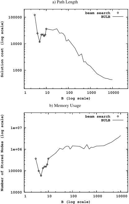
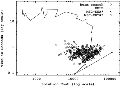
Our �rst benchmark domain was the N-Puzzle, as already described in the context of Table 1. Beam search solved all problem instances of small N-Puzzles with a small average path length and did so in fractions of a second. It is therefore not surprising that neither DB nor BULB signi�cantly improved on beam search for N smaller than 48. The situation was different for the 48-Puzzle. DB did not signi�- cantly improve on beam search for the 48-Puzzle either. On the other hand, BULB was able to solve all problem instances with a beam width of 10,000 while beam search was only able to solve all problem instances with beam widths of 10 or smaller. BULB was able to �nd paths of average length 440 with this beam width while beam search was only able to �nd paths of average length 11,737 with beam widths that allowed it to solve all problem instances (for B = 5, which is not shown in Table 1). Thus, BULB was able to reduce the path length or, synonymously, solution cost by a factor of about 25. At the same time, the average runtime of BULB was still on the order of 30 seconds on a Pentium 4 PC clocked at a 2.2 GHz. Figure 5 contains detailed data points about BULB. Since BULB generates states in exactly the same order as beam search, the graphs of BULB simply extend the ones of beam search to larger beam widths. For the 80-Puzzle and a memory capacity of 3,000,000 states, there was no beam width that allowed beam search to solve all 50 random problem instances but BULB was able to solve them for a wide range of beam widths. The smallest average runtime of BULB with a beam width that solved all problem instances was about 12 seconds. It was obtained with a beam width of 6 and resulted in an average path length of about 181,000. A larger beam width of 20,000, that still solved all problem instances, increased its average runtime to about 120 seconds but reduced the average path length to 1,130, which is less than 5 times the shortest path length. Figure 6 shows that BULB was also able to improve the average path length of two multi-state commitment search methods for the 48-Puzzle by at least one order of magnitude with an average runtime of only about 20 seconds. These alternatives to beam search are MSC-KWA* [Furcy and Koenig, 2005], a combination of KWA* [Felner et al., 2003] and MSC-WA* [Kitamura et al., 1998], and MSC-KRTA* [Furcy, 2004], a combination of KWA* [Felner et al., 2003], MSC-WA* [Kitamura et al., 1998] and RTA* [Korf, 1990].
| B | Path Length | Generated States | Stored States | Runtime (Seconds) | Problems Solved |
| 1 | N/A | N/A | N/A | N/A | 0 % |
| 5 | 37,775.12 | 730,901 | 188,860 | 0.306 | 68 % |
| 10 | 33,489.26 | 1,261,982 | 334,850 | 0.581 | 46 % |
| 50 | 8,468.59 | 1,619,300 | 423,103 | 0.900 | 68 % |
| 100 | 4,629.57 | 1,784,654 | 462,443 | 1.012 | 70 % |
| 500 | 1,363.59 | 2,632,408 | 678,792 | 1.855 | 74 % |
| 1,000 | 831.90 | 3,196,242 | 824,784 | 2.388 | 58 % |
| 5,000 | N/A | N/A | N/A | N/A | 0 % |
4.2 Towers of Hanoi
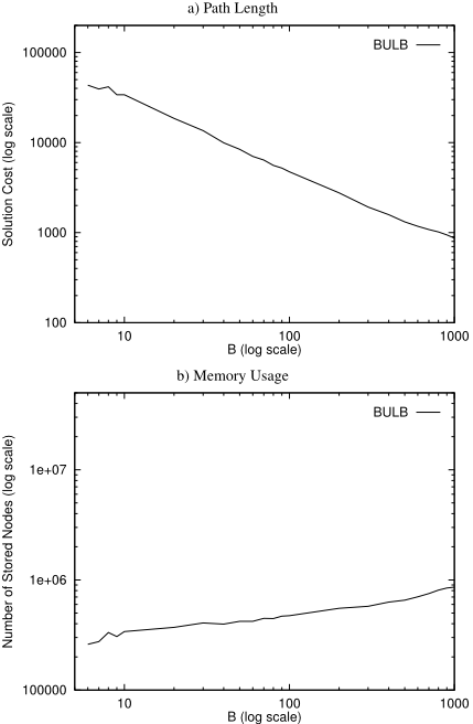
Our second benchmark domain was the 4-Peg Towers of Hanoi. We created 50 random problem instances with 22 disks in which the goal state had all disks stacked on one peg. We set the memory capacity to 1,000,000 states and used a pattern database similar to that of [Felner et al., 2004] as the heuristic function. Table 3 shows that, similarly to the 48-Puzzle, beam search with large beam widths solved many problem instances, and the average length of the paths found was short. However, there was no beam width that allowed beam search to solve all 50 random problem instances (which is the reason why Figure 7 contains no graphs for beam search) but BULB was able to solve them for a wide range of beam widths. The smallest average runtime of BULB with a beam width that solved all problem instances was about 1.5 seconds. It was obtained with a beam width of 40 and resulted in an average path length of about 10,000. A larger beam width of 1,000, that still solved all problem instances, increased its average runtime to about 7 seconds but reduced the average path length to about 870. Figure 7 contains detailed data points about BULB.
4.3 Rubik's Cube
Our third benchmark domain was the Rubik's Cube. We created 50 random problem instances in which the goal state was the original con�guration of the cube. We set the memory capacity to 1,000,000 states and used the pattern databases from [Korf, 1997] as the heuristic function. Beam search was only able to �nd paths of average length 55.18 with beam widths that allowed it to solve all problem instances (for B = 7, 000, which is not shown in Table 4), which is similar to the average path length found by a recent powerful Rubik's Cube solver based on macro-operators, even though this Rubik's Cube solver uses both a larger number of pattern databases to build the macro-operators and a post-processing step on the paths it �nds [Hern·adv¤olgyi, 2001]. Beam search solved all 50 problem instances for several beam widths but BULB was able to solve them for all tested beam widths. BULB with a beam width of 30,000 solved all problem instances and found an average path length of 30.14 with an average runtime of about 40 seconds. This average path length is already smaller than the one of the Rubik's Cube solver mentioned above, even though BULB is a domain-independent search method without any pre- or post-processing and used only about 120
| B | Path Length | Generated States | Stored States | Runtime (Seconds) | Problems Solved |
| 10 | 53,909.26 | 7,146,960 | 539,084 | 14.965 | 38 % |
| 50 | 3,882.35 | 2,570,677 | 194,036 | 5.224 | 98 % |
| 100 | 1,679.76 | 2,223,466 | 167,795 | 4.349 | 98 % |
| 500 | 394.84 | 2,596,065 | 196,182 | 5.168 | 100 % |
| 1,000 | 259.80 | 3,398,726 | 257,058 | 6.798 | 98 % |
| 5,000 | 78.02 | 4,895,297 | 373,602 | 9.977 | 100 % |
| 10,000 | 52.33 | 6,332,050 | 486,767 | 13.087 | 98 % |
| 50,000 | 21.40 | 10,848,794 | 866,741 | 23.256 | 10 % |
| 100,000 | N/A | N/A | N/A | N/A | 0 % |
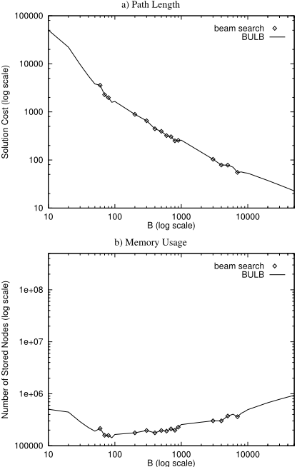
MBytes of memory in our experiments (86 MBytes for the pattern database and 32 MBytes for the hash table). BULB with a beam width of 40,000 found a path of length 25.78 with an average runtime of about 2 minutes. A larger beam width of 50,000, that still solved all problem instances, increased its average runtime to about 7 minutes but reduced the average path length to about 22.74. Figure 8 contains detailed data points about BULB.
5 RelatedWork
Existing variants of beam search differ from BULB in that they either 1) use no backtracking at all or 2) use chronological backtracking. In the �rst category, diversity beam search [Shell et al., 1994] deals with imperfect heuristic values by introducing diversity at all levels of the search tree. It differs from BULB in that it is incomplete and requires additional knowledge to measure the level of dissimilarity among states. Divide-and-conquer beam search [Zhou and Hansen, 2004] does not store all of the beam in memory. Instead, it purges some of its slices from memory and uses a divide-and-conquer strategy to reconstruct the path after it �nds a goal state, which makes backtracking impossible, at least on the parts of the beam that have been purged from memory. In the second category, band search [Chu and Wah, 1992] is the search method most similar to BULB. It differs from BULB in that it extends beam search with chronological backtracking and is designed for search trees. It does not detect loops and therefore performs best for small search problems. Complete anytime beam search [Zhang, 1998] does not extend beam search but depth-�rst search. It uses chronological backtracking (with a beam width of one) while iteratively weakening its pruning rule. Like all depth-�rst search methods, it performs best on �nite trees of shallow depths with large goal densities (such as travelling salesperson problems), which are very different from our benchmark domains.
6 Conclusion
In this paper, we developed BULB (Beam search Using Limited discrepancy Backtracking), a memory-bounded search method that generalizes beam search to beam search with backtracking, limited discrepancy search to beam widths larger than one, and breadth-�rst search to beam widths smaller than in�nity. BULB makes beam search complete (provided that there is suf�cient memory to store the beam along a shortest path from the start state to a goal state), tends to �nd shorter paths than beam search because it is able to use larger beam widths without running out of memory, and can be transformed into an admissible anytime algorithm, for example, by letting it continue its search after it has found a path, resulting in an anytime extension of beam search that is similar in spirit to the anytime extension of WA* described in [Hansen et al., 1997]. BULB outperformed beam search and variants of WA* in our experiments, solved all of our test problems for the 80-Puzzle, and resulted in a state-of-theart Rubik's Cube solver without any pre- or post-processing, even though it is a domain-independent search method. It is future work to enhance BULB with more complex variants of beam search, for example, variants that change the beam width during the search. It is also future work to enhance BULB with more complex variants of backtracking, for example, variants that give a higher priority to decisions close to the top of the search tree than decisions close to the bottom of the search tree, variants that use depth-bounded discrepancy search [Walsh, 1997] or variants that calculate the discrepancies differently.
@inproceedings{ijcai2005p50,
  title     = {Limited Discrepancy Beam Search},
  author    = {Furcy, David and Koenig, Sven},
  booktitle = {Proceedings of the Nineteenth International Joint Conference on
               Artificial Intelligence, {IJCAI-05}},
  publisher = {International Joint Conferences on Artificial Intelligence},
  editor    = {Leslie Pack Kaelbling and Alessandro Saffiotti},
  pages     = {125--130},
  year      = {2005},
  url       = {https://ijcai.org/proceedings/2005/50},
}
TY - CPAPER TI - Limited Discrepancy Beam Search AU - Furcy, David AU - Koenig, Sven T2 - Proceedings of the Nineteenth International Joint Conference on Artificial Intelligence, IJCAI-05 PB - International Joint Conferences on Artificial Intelligence PY - 2005 SP - 125 EP - 130 UR - https://ijcai.org/proceedings/2005/50 ER -Copied
Machine-readable versions of this paper, for tools and AI agents:





