
Limited Discrepancy Search
Proceedings of the Fourteenth International Joint Conference on Artificial Intelligence. Constraint Satisfaction. Pages 607-614.
© 1995 International Joint Conferences on Artificial Intelligence
Abstract
Many problems of practical interest can be solved using tree search methods because carefully tuned successor ordering heuristics guide the search toward regions of the space that are likely to contain solutions. For some problems, the heuristics often lead directly to a solutionbut not always. Limited discrepancy search addresses the problem of what to do when the heuristics fail. Our intuition is that a failing heuristic might well have succeeded if it were not for a small number of "wrong turns" along the way. For a binary tree of height d, there are only d ways the heuristic could make a single wrong turn, and only d( d; 1 l ways it could make two. A small number of wrong turns can be overcome by systematically searching all paths that differ from the heuristic path in at most a small number of decision points, or "discrepancies." Limited discrepancy search is a backtracking algorithm that searches the nodes of the tree in increasing order of such discrepancies. We show formally and experimentally that limited discrepancy search can be expected to outperform existing approaches.
- [Cheng and Smith, 1994] C. Cheng and S. Smith. Gen- erating feasible schedules under complex metric con- straints. In Proc. of the Twelvth National Conference on Artificial Intelligence, 1994.
- [Crawford and Auton, 1993] J. Crawford and L. Auton. Experimental results on the crossover point in satisfi- ability problems. In Proc. 11th AAAI, 1993.
- [Crawford and Baker, 1994] J. Crawford and A. Baker. Experimental results on the application of satisfiabil- ity algorithms to scheduling problems. In Proc. 12th AAAI, 1994.
- [Harvey, 1994] W . Harvey. Search and job shop schedul- ing. Technical Report CIRL TR 94-1, CIRL, Univer- sity of Oregon, 1994.
- [Harvey, 1995] W. Harvey. Nonsystematic Backtracking Search. PhD thesis, Stanford University, 1995.
- [Langley, 1992] P. Langley. Systematic and nonsystem- atic search strategies. In Artificial Intelligence Plan- ning Systems: Proceedings of the First International Conference, 1992.
- [Smith and Cheng, 1993] S. Smith and C. Cheng. Slack- based heuristics for constraint satisfaction scheduling. In Proc. of the Eleventh National Conference on Ar- tificial Intelligence, 1993.
- [Vaessens et al., 1994] R. Vaessens, E. Aarts, and J. Lenstra. Job shop scheduling by local search. Tech- nical Report COSOR 94-05, Eindhoven University of Technology, 1994.
- [Wilkins, 1988] D. Wilkins. Practical Planning: Ex- tending the Classical AI Planning Paradigm. Morgan Kaufman, San Mateo, California, 1988.
References were extracted automatically from the PDF and may contain errors.
Full text extracted automatically from the PDF; figures, tables and equations may differ. The PDF is the version of record.
1 Introduction
In practice, many search problems have spaces that are too large to search exhaustively. One can often find solu tions while searching only a small fraction of the space by relying on carefully tuned heuristics to guide the search toward regions of the space that are likely to contain solutions. For many problems, heuristics can lead di rectly to a solution-most of the time. In this paper, we consider what to do when the heuristics fail.
We will focus our attention on procedures for tree search. Our objective is simple: For search problems with heuristically ordered successors, we will develop a search procedure that is more likely to find a solution in any given time limit than existing methods such as chronological backtracking and iterative sampling [Lan gley, 1992]. The outline of this paper is as follows: In the next section, we discuss existing algorithms. Lim ited discrepancy search (LDS) is introduced in Section 3 and compared to existing techniques in Section 4. We discuss variations of LDS that we believe will be useful for solving realistic problems in Section 5. We conclude by presenting our experimental results in Section 6.
2 Existing Strategies
Consider a tree search problem for which the succes sor ordering heuristic is so good that it almost always leads directly to a solution. Such problems are com mon both in practice and in areas of AI research such as planning and scheduling [Smith and Cheng, 1993; Wilkins, 1988]. If the heuristic is good enough, one might be satisfied with an algorithm that follows the heuristic and just gives up if the heuristic fails to lead to a solu tion, an algorithm we will call "1-samp" [Harvey, 1994; Smith and Cheng, 1993]. If the performance of 1-samp is not satisfactory, however, one is confronted with the question of what search algorithm to use instead. Itera tive sampling and backtracking are two candidates.
2.1 Iterative Sampling
Iterative 6ampling [Langley, 1992], or i6amp, is the sim ple idea of following random paths, or probes, from the root until eventually a path that leads to a solution is discovered. At each node on a path, one of the succes sors is selected at random and expanded. Then one of its successors is selected at random, and so on until a goal node or dead end is reached. If the path ends at a dead end, isamp starts a new probe, beginning again at the root.
Since the algorithm samples with replacement, there is a uniform chance of finding a goal node on any particular probe. Provided that there is a goal node somewhere in the space, it follows that the probability of find a goal node increases uniformly toward 1 as the number of probes grows without limit.
Iterative sampling has been shown to be effective on problems where the solution density is high [Crawford and Baker, 1994], but its performance as a fallback pro cedure for 1-samp is questionable because it ignores the successor-ordering heuristic. If the heuristic were the key to solving the problem despite a low solution density, one would not expect iterative sampling to be effective. 1
2.2 Backtracking
An alternative fallback procedure is simply to backtrack chronologically when 1-samp fails. Our experiments in Section 6 with scheduling show that this approach pro vides little improvement over 1-samp itself, and the anal ysis of mistakes provides an explanation [Harvey, 1995]. There is a reasonable chance that, somewhere early in 1-samp's path, it made a mistake by selecting a succes sor that had no goal nodes in the entire subtree below it. Once this early mistake is made and the successor's sub tree is committed to, none of the subsequent decisions makes any difference.
If the subtree below a mistake is large, chronological backtracking will spend all of the allowed run time ex ploring the empty subtree, without ever returning to the last decision that actually matters. If one is counting on the heuristics to find a goal node in a small fraction of the search space, then chronological backtracking puts a tremendous burden on the heuristics early in the search and a relatively light burden on the heuristics deep in the search. Unfortunately, for many problems the heuristics are least reliable early in the search, before making de cisions that reduce the problem to a size for which the heuristics become reliable. Because of the uneven re liance on the heuristics, it is unlikely that chronological backtracking is making the best use of the heuristic in formation.
3 Discrepancies
Let us return to the search problems for which the suc cessor ordering heuristic is a good one. Our intuition is that, when 1-samp fails, the heuristic probably would have led to a solution if only it had not made one or two "wrong turns" that got it off track. It ought to be pos sible to systematically follow the heuristic at all but one decision point. If that fails, we can follow the heuristic at all but two decision points. If the number of wrong turns is small, we will find a solution fairly quickly using this approach.
We call the decision points at which we do not fol low the heuristic "discrepancies." Limited discrepancy search embodies the idea of iteratively searching the space with a limit on the number of discrepancies al lowed on any path. The first iteration, with a limit of zero discrepancies, is just like 1-samp. The next iteration searches all possibilities with at most one discrepancy, and so on.
The algorithm is shown in Figure 1. We will assume the search tree is binary. SUCCESSORS is a function that returns a list of the either zero or two successors, with the heuristic preference first.
In Figure 1, z is the discrepancy limit. We iteratively call LDS-PROBE, increasing z each time. LDS-PROBE does a depth-first search traversal of the tree, limiting the number of discrepancies to z. When eventually z
1 We have experimented with biasing the random selec tion of successors according to the heuristic, but our results suggest this is not a viable approach [Harvey, 1995].
LDS-PROBE{node, k) 1 if GOAL-P{node) return node 2 s t- SUCCESSORS (node) 3 if NULL-P{s) return NIL 4 if k = 0 return LDS-PROBE{FIRST(s), 0) 5 else 6 result+- LDS-PROBE{SECOND{s), k- 1) 7 if result =P NIL return result 8 return LDS-PROBE{FIRST(s), k) LDS(node) · 1 for z t- 0 to maximum depth 2 result t- LDS-PROBE{node, z) 3 if result =P NIL return result 4 return NILreaches d, the maximum depth of the tree, LDS-PROBE searches the entire tree exhaustively. Thus the search is guaranteed to find a goal node if one exists and is guaranteed to terminate if there are no goal nodes.
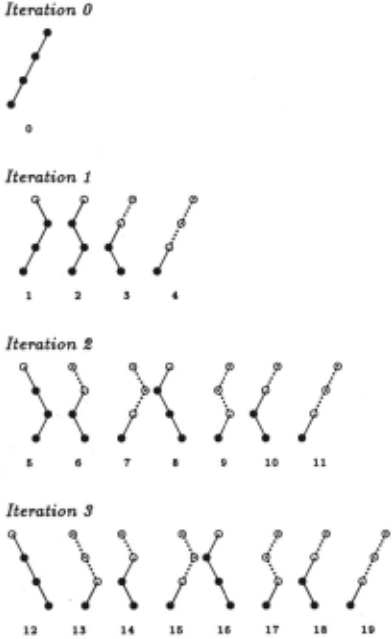
Since each iteration of LDS-PROBE limits the num ber of discrepancies to z instead of restricting the search to those nodes with exactly z discrepancies, iteration n reexamines the nodes considered by previous iterations {see Figure 2). As with other iterative techniques, how ever, the final iteration is far and away the most expen sive and the redundancy is therefore not a significant factor in the complexity of the search.
Figure 2 shows a trace of LDS exhaustively searching a full binary tree of height three. The heuristic orders nodes left to right. The twenty pictures show all the paths to depth three, in order. The dotted lines and open circles represent nodes that were not backtracked over since the previous picture, so the trace can be followed by examining at the pictures in sequence. Counting all the black circles gives the total number of nodes expanded in the search, forty.
In general, the number of nodes expanded by LDS with a discrepancy limit of z is bounded by dz+l {for iteration z, there are at most dz fringe nodes, with each path to a fringe node expanding at most d nodes). If d is large, the cost of any single iteration dominates the summed costs of the preceding ones.
4 Comparison with existing methods
In practice, of course, we will typically not have time to search the space exhaustively. We would therefore like to know the likelihood of finding a solution, using the various methods, in the amount of time we are actually willing to wait. We will make this question precise by formalizing what we mean for the heuristic to make a "wrong turn."
4.1 Wrong Turns
For simplicity, we will consider only the case of a full binary tree. The two children of each choice point are assumed to be in the order of heuristic preference. We will further assume that if a choice point has a goal node in the subtree below it, then with probability p (the heuri8tic probability) its first child has a goal node in its subtree. If the first child does not have a goal, the other child must have a goal since the choice point has only two children. In this case the heuristic has made a wrong turn by putting the children in the "wrong" order.
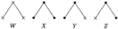
The notion of a wrong turn is closely related to the mistake probability. We define a bad node to be a node that does not have any goal nodes in its subtree. We define a mi8take to be a bad node whose parent is not bad. The mi8take probability, m, is the probability that a randomly selected child of a good node is bad [Harvey, 1995]. If the heuristic orders successors randomly, the heuristic probability is the complement of the mistake probability, p = 1 - m. If the heuristic does better than random selection, p > 1-m.
Figure 3 shows the four possibilities for a node and its children. An X indicates a bad node, a solid dot a good node. In the figure, p is the probability that a node is in class X or Y (the two classes with good left children) given that it is not in class W (the only class where the parent is bad). The mistake probability m is one half the probability that a node is in class Y or Z (the classes with one mistake child) given that it is not in class W.
Experimentally, it appears that m is l$enerally fairly constant throughout many search trees lHarvey, 1995].
~n order to simplify our analyses, we will assume that p 1s constant as well, although the experimental evidence is that p tends to increase somewhat as we search the tree because most heuristics are more accurate at deep nodes than at shallow ones.
The chance of finding a solution on a random path to depth d (i.e., using isamp) is simply (1- m)d. Using heuristics and assuming a constant p, 1-samp has prob ability pd of finding a solution on its one and only path.
This observation allows us to estimate p by running 1samp on a large training set of problems from the domain of interest. Let 8 be the success rate of 1-samp on the training set. Since the probability of success for 1-samp is pd, we have p = 8 1 1 d. If 8 is small, the training set may have to be impractically large to get a reliable estimate . For some problems, though, 8 is not small. Heuristics de veloped for job shop scheduling have been shown to yield a probability 8 that is nearly one for small research prob lems [Smith and Cheng, 1993]. We have found in earlier experimental work on the same problems [Harvey, 1994] that even standard CSP heuristics can yield a success rate of about 75%. On larger scheduling problems [Vaessens et al., 1994] the success rate of 1-samp is less, but more sophisticated heuristics from operations research keep 1samp competitive with other search techniques [Cheng and Smith, 1994].
4.2 Theoretical results
Given specific values for m and for p, Figures 4 and 5 show the theoretical probability of success as a func tion of time for iterative sampling (isamp), chronologi cal backtracking ( DFS), and limited discrepancy search (LDS) for various heuristic probabilities p. 2 The graphs show the probability of finding a solution in some num ber of probes i, where we define a probe to be a search until a dead end is reached for isamp or LDS, or simply a search of an additional d nodes for DFS. The num ber of probes is limited by the height of the tree be cause the combinatorics of solving the problem beyond the one-discrepancy limit are intractable. The analyses are bi.ased toward DFS because depth-first search is given the highest of the heuristic probabilities shown in each figure.
Figure 4 shows results for a problem of height 30, with a mistake probability m of 0.2. The problem has about a billion fringe nodes of which a few more than a million are goals. 3 With a solution density of 1/1000, we would expect iterative sampling to sample about 500 fringe nodes before finding a solution (807, to be exact). 4 By many accounts, a problem with a solution density of 0.001 is a fairly easy problem. It takes only 807 · 30 = 24, 210 nodes, on average, to find a solution us ing iterative sampling. The expected number of probes is slightly more than the number of probes required to have a 50% chance of finding a solution, 560 · 30 = 16, 800. 5
2 The combinatoric manipulations underlying these figures are quite involved and appear elsewhere [Harvey, 1995].
3 The number of goals is (2- 2m)d.
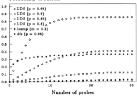
In practice, we may be interested in the number of nodes required to find a solution with a higher probabil ity of success. The number of nodes required by iterative sampling for a success probability of 0.8 on this problem is 1300 · 30 = 39, 000. Compare this to the performance of limited discrepancy search. For p = 0.95, LDS has probability of success 0.8 with just eleven probes, or 990 nodes. The savings, nearly a factor of forty, depends on the heuristic to order successors correctly seven out of eight times when one of the successors is a mistake.
For p = 0.8 = 1-m, the heuristic orders the successors correctly half the time, no better than random selection. The p = 0.8 curve in the figure {almost completely ob scured by the isamp curve) shows that the performance of LDS is slightly worse than iterative sampling under these conditions. For p = 0.85, 0.9, and 0.95 the heuris tic orders nodes correctly five, six, and seven out of eight times. The curves show that the expected performance of LDS increases dramatically with the better p.
The DFS curve for p = 0.95 rises only marginally above the probability 0.21 that its first fringe node is a goal. 6 The futility of DFS is even clearer in the deeper search shown in Figure 5.
The problem of Figure 5 has height 100, and approxi mately 10 30 nodes. The density of solutions form= 0.1 is about 2.6 x 10- 5 · Iterative sampling needs 26,096 probes {2.6 million nodes) to have a 50% chance of suecess. If, as in the earlier problem, the heuristic orders nodes correctly seven out of eight times (p = 0.975 for m = 0.1), LDS has a similar chance with just twenty probes {2,000 nodes), a savings of three orders of mag nitude over iterative sampling. The savings is similar if a success probability of 0.8 is desired instead.
4 The expected number of probes is 1/(1- m)a.
5 For example, the expected number of coin flips before getting heads is two, whereas it takes only a single coin flip to have probability 0.5 of getting heads. The number of probes required to achieve a given success probability 11 is log(1-·) log(1-(1-m)a) ·
6 The probability that the first fringe node examined by DFS is a goal is simply pd.
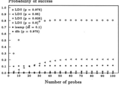
For higher probabilities of success, the three orders of magnitude savings is more doubtful, though perhaps not as doubtful as the graph seems to suggest. The one discrepancy iteration ends after 101 probes. The later probes of the one discrepancy iteration have much of their paths in common, so the likelihood that one of these later probes succeeds given that the others failed is small. After 101 probes, though, the two discrepancy iteration begins to explore "fresh" paths again. Consequently, we would expect the LDS curve to rise steadily once again where the graph leaves off. 7
5 Variations and Extensions
The reason we have focused on analyzing the early iter ations of limited discrepancy search is that we believe in practice they are the only iterations that matter. Earlier, we argued on intuitive grounds that they would be more important than the later iterations. We will now take the position that in practice the later iterations don't matter at all. The reason is that if the objective is to maximize the probability of finding a solution in a given number of nodes, there are always better things to do than use those nodes on later iterations of limited dis crepancy search.
This section discusses a few of the more promising ·choices. Since some involve combinations with other techniques and others depend on search space properties that are difficult to quantify, this discussion will be less precise than that of earlier sections. Here, we will view limited discrepancy search as a tool that can be used in combination with other techniques to craft an effective search procedure for a given real world problem.
7 As remarked earlier, we are unfortunately unable to ver ify this essentially theoretical claim because the combina torics overwhelm us.
5.1 Variable Reordering
Constraint satisfaction problems and SAT problems are formulated as tree search by fixing an order for the vari ables to be instantiated or determining the order dynam ically as the search progresses. In either case, a node in the search tree is a choice point for the possible instan tiations of a particular variable. If an effective heuristic does not solve the problem with a limit of one discrep ancy for some chosen variable order, it may still solve the problem with one discrepancy given a different variable order. The "wrong turn" instantiations that the heuris tic makes on the first variable order may even follow from unit propagation on the second. This suggests the simple technique of repeating the one discrepancy iteration of Los with different variable orders. When variable order is determined dynamically, it may suffice simply to begin the search with a different variable on each iteration. A similar technique improves the efficiency of depth-first search as well (see Section 6).
5.2 Using Different Heuristics
If multiple heuristics exist for a particular problem, one can try repeating the one- or two-discrepancy limit iter ations of LOS with different heuristics. If one heuristic is unlucky and makes more than two wrong turns on a given problem, some other heuristic may be luckier. In general, what is hard for one heuristic may not be hard for another. Los is an effective way to give one heuristic a reasonable chance before switching to another.
5.3 Combining LDS with Bounded Backtrack Search
Los can also be combined with bounded backtrack search (BBS) [Harvey, 1995] to produce an algorithm that does not count "small" discrepancies (those that fail quickly) toward the discrepancy limit. This algo rithm can also be viewed as modifying the heuristic to avoid choices that can be seen to fail using a fixed looka head. (The algorithm itself appears in Appendix A.)
The combined LoS-BBS algorithm outperforms both LOS and BBS on job shop scheduling problems. In fact, LOS-BBS appears to be the algorithm of choice among all systematic backtracking strategies in this domain. There is a compelling theoretical argument for this. Many mis takes result in quick, if not immediate, failures. If a heuristic makes few wrong turns to begin with, it makes even fewer wrong turns that exceed the backtrack bound. Adding a bounded backtrack enables limited discrepancy search to discover solutions with a discrepancy limit of no more than the number of wrong turns that actually exceed the backtrack bound, potentially reducing the number of required iterations. Since the cost of each LOS iteration grows by a factor of d, the savings can be substantial. The added cost of the backtrack bound is relatively insignificant. Adding a backtrack bound of one node can cost at most a factor of 2. A backtrack bound of l costs at most a factor 2 1 and, for small l, is likely to be cheaper than the cost of an additional iteration. This upper bound is conservative since the heuristic, by assumption, makes few mistakes.
5.4 Local Optimization Using LDS
For problems like scheduling, LOS can also be used to search the neighborhood of an existing solution. The one discrepancy iteration ofLoS is modified to begin fol lowing the path of the previous best solution instead of following the heuristic. At the depth of the discrepancy, the algorithm diverges from the previous solution and follows the heuristic for the remaining decisions. If the path ends in a solution that is better than the previ ous best, it can be adopted immediately or stored as a contender for the basis of the next iteration.
This variation of LOS requires some measure of the "goodness" of a solution. For scheduling problems, the schedule length is often . the appropriate measure. Searching for a schedule that takes less than time L, if successful, produces a schedule that takes time L'. A set of standard Los iterations can be repeated with the lower time bound L', or the optimization variant of LOS can be applied to consider variations of the previous schedule that differ by at most one discrepancy. 8
5.5 Non-Boolean problems
Finally, we should at least comment on the possible ex tension of Los to constraint-satisfaction problems in volving variables with domain sizes larger than 2. Al though we have focussed on Boolean problems in this paper (in part because the most natural encoding of job shop scheduling problems is Boolean [Smith and Cheng, 1993]), the technique can obviously be applied in a wider setting. There are a variety of choices that will need to be made, however: Should the one-discrepancy search include every alternate value for the variable that vio lates the heuristic, or only the single next most attractive choice? If the number of nodes expanded is to increase by a factor of no more than d on each iteration, we will need to take the latter view.
6 Experimental Results
Our experimental results comparing limited discrep ancy search with chronological backtracking and itera tive sampling are based on a set of thirteen job shop scheduling problems taken from a recent survey of oper ations research techniques [Vaessens et al., 1994]. 9 Each of the problems involves scheduling the tasks that might be involved in producing widgets in a manufacturing set ting: Each job ii needs to be performed on a particular machine 7'14 and takes time ti. There are constaints indi cating that some jobs need to be completed before others can be started, and so on.
The most effective encoding of problems such as these focusses directly on the resource contentions that arise; if two jobs ii and i1c require the same machine, we intro duce a variable Pile indicating whether it is job ii or job i1c that uses the machine first [Smith and Cheng, 1993].
8 Alternatively, the time bound can be adjusted by binary division. A single iteration of LDS, though, is not a decision procedure, so failure to find a schedule for a given time bound is no proof that no such schedule exists.
8 The problems can be obtained by sending a message to o.rlibraryOic.ac.uk.
Because these variables are Boolean, the search space is far smaller than it would be if we were to make the variables the start times of the various jobs themselves.
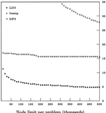
Our experimental work formulated each problem as a CSP with a loose bound on the schedule length. We then iteratively repeated the search, decreasing the bound each time to slightly less than the length of the last schedule found. We recorded the length of the best schedule found as a function of the total number of nodes expanded until reaching a final cutoff of 500,000 nodes per problem (see Figure 6).
Avg. percent above optimal
Node limit per problem (thousands)
Figure 6: Comparison to DFS and iterative sampling.
At any given node cutoff M :::; 500, 000, each algo rithm had completed some number of iterations for each problem, resulting in schedules of various lengths. We evaluated the schedules by these lengths, measuring their percent above the optimal length for each problem. 10 We took the average percent above optimal (a function of M) as the overall measure of the performance of the search algorithms.
In Figure 6, LDS is clearly superior to chronological backtracking and iterative sampling. We chose this par ticular benchmark, though, so that we could also com pare our results with other scheduling research in artifi cial intelligence and operations research. On this bench mark, contemporary OR scheduling programs score in the range 0.45% to 8.31% above optimal [Vaessens et al., 1994]. Although the performance of our implementation does not match the best of these programs, it appears to be in the same range.
Our scheduling implementation uses general CSP heuristics, which are weak by scheduling standards. Relative to the larger pool of programs, our implementa tion appears to be comparable using limited discrepancy search but disastrous using chronological backtracking and iterative sampling. Since limited discrepancy search relies heavily on the heuristics, we expect that the com bination of LDS with the more accurate heuristics of the dedicated scheduling programs would have the best per formance overall. Experiments in this vein are under way.
10 The optimal lengths were taken to be the best reported lengths as of November, 1994.
We also experimented with a variety of nonsystem atic algorithms (Harvey, 1995]. Depth-first search with restarts, iterative broadening, and bounded backtrack search scored 4.9%, 4.6%, and 4.2% above optimal on the benchmark and all outperformed pure limited discrep ancy search slightly (LDS was also 4.9% above optimal).U
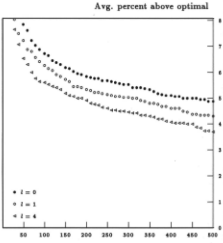
However, since all of these nonsystematic methods rely less on the heuristics than LDS, we believe that LDS is likely to benefit more significantly from future improve ments to the heuristics. As we commented in Section 5.3, limited discrepancy search can also be combined with bounded backtrack search. The results are shown in Fig ure 7. 12
Node limit per problem (thousands)
Figure 7: Adding bounded backtrack improves BBS.
The combination of limited discrepancy with bounded backtrack search had the best performance of all the sys tematic and nonsystematic methods we tested. At 3.68% over optimal, its performance with a four-node backtrack bound is respectable when compared to the dedicated scheduling programs.
11 Although the overall difference of 0.7% between the best and worst of these algorithms may appear slight, it is sub stantial in this domain, since the problems can be expected to become exponentially more difficult as one approaches the crossover point corresponding to optimality [Crawford and Auton, 1993].
12 The parameter l in the figure is the depth of backtrack allowed in checking for heuristics that led to dead ends.
7 Conclusion
We have shown both theoretically and experimentally that limited discrepancy search is an effective way to exploit heuristic information in tree search problems. It is more effective than either chronological backtracking or iterative sampling, and we have attempted to explain why.
The scheduling problems that we used in our experi ments, while large by contemporary research standards, are not large relative to the types and sizes of scheduling problems it would be useful to solve in the real world. Because of the complexity of scheduling, it is likely that the challenge of scaling up from research problems to real world problems will be met more quickly by advances in heuristics than by the evolution of brute force methods. We expect that in the future, techniques that depend on heuristics yet recover gracefully by searching alternatives when the heuristics fail will be the methods of choice for solving real world problems.
Acknowledgement
This work has been supported by the Air Force Office of Scientific Research under contract 92-0693 and by ARPA/Rome Labs under contracts F30602-91-C-0036 and F30602-93-C-00031. The authors would like to thank to Andrew Baker, Ari Jonsson, Jimi Crawford and David Etherington for valuable feedback in the course of this research.
A The combined LDS-BBS algorithm
LB-PROBE(node, k, look)
1 ifGOAL-P(node) return (node,O) 2 s f- SUCCESSORS (node) 3 if k > 0, sf- REVERSE(s) 4 if- 0 5 count f- 0 6 maxheight f- 0 7 for child in s 8 if k = 0 and count ~ 1 break 9 if k > 0 and i = 0 k' f- k - 1 10 else k' f- k 11 (result,height) f- LB-PROBE(child, k', look) 12 maxheight f- MAx(maxheight, 1 + height) 13 if result =f; NIL return (result, 0) 14 if- i + 1 15 if height ~ look, count f- count+ 1 16 return (NIL, maxheight) LDS-BBS(node, look) 1 for z f- 0 to maximum depth 2 (result, height) f- LB-PROBE(node, z, look) 3 if result =f; NIL return result 4 return NIL@inproceedings{ijcai1995p80,
title = {Limited Discrepancy Search},
author = {Harvey, William D. and Ginsberg, Matthew L.},
booktitle = {Proceedings of the Fourteenth International Joint Conference on
Artificial Intelligence, {IJCAI-95}},
publisher = {International Joint Conferences on Artificial Intelligence},
editor = {Chris S. Mellish},
pages = {607--614},
year = {1995},
note = {Constraint Satisfaction},
url = {https://ijcai.org/proceedings/1995/80},
}
TY - CPAPER TI - Limited Discrepancy Search AU - Harvey, William D. AU - Ginsberg, Matthew L. T2 - Proceedings of the Fourteenth International Joint Conference on Artificial Intelligence, IJCAI-95 PB - International Joint Conferences on Artificial Intelligence PY - 1995 SP - 607 EP - 614 UR - https://ijcai.org/proceedings/1995/80 ER -Copied
Machine-readable versions of this paper, for tools and AI agents:





