
Automatic Abstraction in Component-Based Diagnosis Driven by System Observability
Proceedings of the Eighteenth International Joint Conference on Artificial Intelligence. Pages 394-401.
© 2003 International Joint Conferences on Artificial Intelligence
Abstract
The paper addresses the problem of automatic abstraction of component variables in the context of Model Based Diagnosis, in order to produce models capable of deriving fewer and more general diagnoses when the current observability of the system is reduced. The notion of indiscriminability among faults of a set of components is introduced and constitutes the basis for a formal definition of admissible abstractions which preserve all the distinctions that are relevant for diagnosis given the current observability of the system. The automatic synthesis of abstract models further restricts abstractions such that the behavior of abstract components is expressed in terms of a simple and intuitive combination of the behavior of their subcomponents. As a validation of our proposal, we present experimental results which show the reduction in the number of diagnoses returned by a diagnostic agent for a space robotic arm.
- [Autio and Reiter, 1998] K. Autio and R. Reiter. Struc- tural abstraction in model-based diagnosis. In Proc. ECAI98, pages 269-273, 1998.
- [Chittaro and Ranon, 2001] L. Chittaro and R. Ranon. Hierarchical diagnosis guided by observations. In Proc. IJCAI01, pages 573-578, 2001. IJCAI
- [Console and Theseider Dupre, 1994] L. Console and D. Theseider Dupre. Abductive reasoning with ab- straction axioms. LNCS, 810:98-112, 1994.
- [Darwiche, 1998] A. Darwiche. Model-based diagnosis using structured system descriptions. Journal of Ar- tificial Intelligence Research, 8:165-222, 1998.
- [Friedrich, 1993] G. Friedrich. Theory diagnoses: A con- cise characterization of faulty systems. In Proc. IJ- CAI93, pages 1466-1471, 1993. IJCAI
- [Mozetic, 1991] I. Mozetic. Hierarchical model-based diagnosis. Int. Journal of Man-Machine Studies, 35(3):329-362, 1991.
- [Out et al., 1994] D.J. Out, R. van Rikxoort, and R. Bakker. On the construction of hierarchic mod- els. Annals of Mathematics and AI, 11:283-296, 1994.
- [Pagallo and Haussler, 1990] G. Pagallo and D. Haus- sler. Boolean feature discovery in empirical learning. Machine Learning, 5:71-99, 1990.
- [Portinale and Torasso, 1999] L. Portinale and P. Torasso. Diagnosis as a variable assignment problem: a case study in a space robot fault diagnosis. In Proc. IJCAI99, pages 1087-1093, 1999. IJCAI
- [Provan, 2001] G. Provan. Hierarchical model-based di- agnosis. In Proc. DX01, pages 329-362, 2001.
- [Sachenbacher and Struss, 2001] M. Sachenbacher and P. Struss. Aqua: A framework for automated qual- itative abstraction. In Proc. QR01, 2001.
- [Struss et al., 1996] P. Struss, A. Malik, and M. Sachen- bacher. Qualitative modeling is the key to automated diagnosis. In Proc. IFAC96, 1996.
- [Struss, 1997] P. Struss. Fundamentals of model-based diagnosis of dynamic systems. In Proc. IJCAI97, 1997. IJCAI
- [Torasso and Torta, 2002] P. Torasso and G. Torta. Merging indiscriminable diagnoses: an approach based on automatic domains abstraction. In Proc. DX02, pages 43-50, 2002.
References were extracted automatically from the PDF and may contain errors.
Full text extracted automatically from the PDF; figures, tables and equations may differ. The PDF is the version of record.
1 Introduction
System model abstraction has been successf~lly e~ ploited in many approaches to model-based dtagnosts (MBD). The pioneer work of [Mozetic, 1991] and re cent improvements proposed e.g. by [Provan, 2001] and [Chittaro and Ranon, 2001] mostly use abstraction in or der to focus the diagnostic process and thus improve its efficiency. However, (flexible) abstraction has anot~er main benefit, namely to provide fewer and more conetse abstract diagnoses when it is not possible to discriminate among detailed diagnoses. The works by [Console ~d Theseider Dupre, 1994] and [Friedrich, 1993] accomplish this goal by including abstraction axioms in the Domain Theory and using preference criteria based on the ab straction level of diagnoses.
Recently, some authors have aimed at the same goal in a different way, namely automatic abstraction of the system model ([Sachenbacher and Struss, 2001], [Torasso and Torta, 2002]) 1 . If the available observables and/or their granularity are too coarse to distinguish amor,tg ~wo or more behavioral modes of a component, or the dtstmc tion is not important for the considered system, a system model is automatically generated where such behavioral modes are merged into an abstracted behavioral mode. By using the abstracted model for diagnosis there's no loss of (important) information, while the number of re turned diagnoses is reduced, and such diagnoses, by be ing "as abstract as possible", are more understandable for a human.
1 Previously an algorithm for automatic abstraction of
The work presented in this paper aims at extending previous works by introducing automatic abstraction of variables (i.e. components) in the presence of a reduced availability of the number and/or granularity of observ ables. Abstractions based on system observability are particularly relevant in the context of on-board diagno sis. Indeed, it is likely that when a system is operated on board the only available measures are provided by sen sors (which can themselves fail) and taking further mea sures manually is out of question. Moreover, on-board diagnosis is usually constrained by strict time and re sources requirements: using an abstracted system model should yield savings in both the time and the space re quirements of the diagnostic process.
Our proposal requires that abstractions do not cause any loss of diagnostic information (e.g. as in the_ in complete abstractions discussed in [Autio and Reiter, 1998]) or loss of efficiency (e.g. due to increased fan in as pointed out in [Provan, 2001]); moreover, we re strict the mapping from abstract components to their subcomponents to be enough simple and intuitive. In order to exclude all the undesired abstractions we intro duce a precise definition of admissible abstraction, and further restrict the computation of abstractions through cutoff criteria which forbid admissible abstractions that may lead to computational inefficiencies.
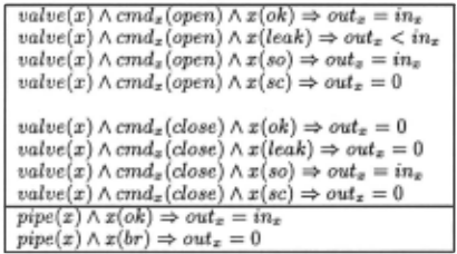
As a running example to illustrate our definitions and algorithms, we will use throughout the pape: the frag ment of hydraulic circuit adapted from [Chtttaro and Ranon 2001] depicted in figure 1 (a); table 1 reports its do~ain theory (valve modes so and sc abbreviate stuck open and stuck closed respectively). Two possible abstractions of such system are shown in figures 1 (b) (where pipe P1 and valve V1 have been abstracted into valve AV1) and 1 (c) (where abstract valve AV1 and pipe P2 have been abstracted into valve AV2). As for experimental validation of our techniques, however, we will present results collected in a larger domain, namely the model of the SPIDER space robotic arm used in [Portinale and Torasso, 1999].
components had been proposed in [Out et al., 1994] for sim pler models describing only normal behavior of the system

The paper is structured as follows. In section 2 we give a formal definition of what we consider an admissible abstract component. In section 3 we describe how the declarative notions introduced in 2 can be implemented computationally. In section 4 we present experimental results collected in the SPIDER robotic arm domain. Finally, in section 5 we compare our work to related papers and make some concluding remarks.
2 Abstractions Defined
We first report formal definitions of system model, diag nostic problem and diagnosis.
Definition 2.1 A System Description (SD) is a 3-tuple (V, DT, Q) where:
- V is a set of discrete variables partitioned in the fol lowing sorts: CXT (inputs), COMPS (components), STATES (endogenous variables), OBS (observables); DOM(v) is the finite domain of variable v E V
- DT (Domain Theory) is an acyclic set of Horn clauses defined over V representing the behavior of the system {under normal and abnormal conditions); we require that, given an instantiation of COM P S and C XT, the DT derives exactly one value for each other variable
- 9 (Causal Graph) is a DAG whose nodes are in V rep resenting the causal structure of the system; whenever a formula N1(bm1) 1\ ... I\ Nk(bmk) => M(bmt) appears in DT, nodes N1 through Nk are parents of M in the graph
It is worth noting that the fact that g is restricted to be a DAG does not mean that the system model is a tree in the sense e.g. of [Darwiche, 1998]; since we allow the existence of multiple directed paths between two nodes the associated jointree may well be cyclic. The DAG re striction just forbids feedback loops in the causal graph, which is a common assumption in approaches which deal with dynamic systems only if they are amenable to state based diagnosis ([Struss, 1997]).
Example 2.1 Note that the System Description for the running sample system given in table 1 is expressed in a slightly different formalism than the one described in our definition, due to the use of equations and disequa tions on the right-hand side offormulas. However, it can be easily mapped to our formalism by modeling in., and m.tt., as discrete STATES variables by using qualitative deviations ([Struss et al., 1996]); thus, for example, for mula:
valve(x) 1\ cmd.,(open) 1\ x(ok) =>aut.,= in., is mapped to a set of three formulas:
in.,( ( +, 0)) 1\ cmd.,(open) 1\ x(ok) =>aut.,((+, 0}) in.,((+,-}) 1\ cmd.,(open) 1\ x(ok) =>aut.,((+,-}) in.,((O, -}) 1\ cmd.,(open) 1\ x(ok) => aut.,((O, -})
where v( ([val], [~val]}) means that variable v has a value with sign [val] and its deviation from the nominal value has sign [~val]. In the rest of the examples we continue to use the notation of [Chittaro and Ranon, 2001] simply because it is more compact. 0
Definition 2.2 A diagnostic problem is a 3-tuple DP = (SD, OBS, CXT} where SD is the System Description, OBS is an instantiation of OBS and CXT is an in stantiation of CXT
Definition 2.3 Given a diagnostic problem DP = (SD, OBS, CXT} an instantiation D = {C1 (bmi), ... , Cn(bmn)} of COMPS is a di agnosis for D P iff:
VM(val) E OBS DT U CXT U D f- M(val) 2
As noted in the introduction, there are real scenar ios where not all the observables OBS are available and/or their granularity is reduced. We identify the available observables with a set OBSAv ~ OBS; we also assume that a granularity mapping II is given s.t. II(M(val)) maps an instantiation of M E OBSAv to a possibly more abstract instantiation M(aval). If VM E OBSAv, Vval E DOM(M) : II(M(val)) = M(val) then there is no loss of granularity at all; in this particu lar case we denote II with IIid· For example, in figure 1 (a), OBSAv = OBS = {autl,in2,aut}; in 1 (b), OBSAv = {in2,aut} and in 1 (c), OBSAv = {aut}; as for II we may consider a situation where aut., = in., and aut., < in., have been mapped to a coarser value out., i 0. The important point about OBSAv and II is that these reductions of the observability of the sys tem can cause the model to become less discriminant and thus different faults of the same component and/or of different components to become indiscriminable. The following definition introduces the notion of indiscrim inability among instantiations of subsets of COM P S.
2 This definition of diagnosis is fully abductive; how ever results presented in this paper apply equally well to consistency-based diagnosis
Definition 2.4 Let SCOMPS be a subset ofCOMPS, OBSAv the set of available observables and II a granularity mapping. We say that two instan tiations SCOMPSl, SCOMPS2 of SCOMPS are (OBSAv, II)-indiscriminable iff for any instantiation CXT of C XT and any instantiation OTHERS of COMPS\SCOMPS the following holds 3 :
II(tclosureonsAv (OTHERS U SCOMPSl)) = II(tclosureonsAv (OTHERS U SCOMPS2))
Note that the (OBSAv,II)-indiscriminability relation induces a partition into ( 0 B S AV, II)-indiscriminability classes of the set of possible instantiations of SCOM PS. Also note that, when jSCOMPSj = 1, indiscriminabil ity coincides with the indistinguishability among behav ioral modes introduced in [Torasso and Torta, 2002].
Example 2.2 In the abstraction example of figure 1 (b), under context cmd = open in discriminable in stances of P1, V1 are grouped in the following sets: C1 = { (ok, ok), (ok, so)} (which derive in2 = in); C2 = { (ok, leak)} (which derives in2 < in); C3 = { (ok, sc), (br, ok), (br, leak), (br, so), (br, sc)} (which de rive in2 = 0). By also considering context cmd =close, set C1 is further split in two distinct sets: C11 = { (ok, ok)} (which derives in2 = 0) and C12 = { (ok, so)} (which derives in2 = in). If in a specific diagnostic prob lem we observe, for instance, in2 = 0 given cmd =open, the set of diagnoses is given by C3 4 . 0
For now, just note how this notion of indiscriminabil ity is the basis for any potential abstraction. If, in deed, two instantiations SCOMPSl and SCOMPS2 of SCOMPS ~ COMPS are indiscriminable, this means that whenever SCOMPSl U OTHERS is a diagnosis for a given DP, SCOMPS2 u OTHERS is another, indiscriminable, diagnosis for D P.
We now introduce a weak notion of abstraction where, as it is common in structural abstractions, abstract com ponents are recursively built bottom-up starting with the primitive components.
Definition 2.5 Given a set COMPS = {C1 , ... ,Cn} of component variables, a components abstraction map ping AM of COMPS defines a set COMPSA = {AC1 , ... , ACm} of discrete variables {abstract compo nents) and associates to each ACi E COM P SA one or more Cj E COMPS (subcomponents of ACi) s.t. each component in COMPS is the subcomponent of exactly one abstract component. Moreover, AM associates, to each abstract component AC a definition def AC, which is a characterization of the behavioral modes of AC in terms of the behavioral modes of its subcomponents. More precisely, an abstract component and its definition are built hierarchically as follows:
3 Given an instantiation COMPS of COMPS we denote with tclosureoasAv (COMPS) the set of instantiations of variables in OBSAv derived from (DT U CXT U COMPS)
4 There are IC31 = 5 indiscriminable diagnoses; 2 of them, namely (ok, sc) and (br, ok), can be regarded as preferred diagnoses since they involve only one fault
- if C E COM P S, AC is a simple abstract compo nent if its definition def AC associates to each abm E DOM(AC) a formula defabm C(bmt) V ... V C(bmk) s.t. bm1 , ... ,bmk E DOM(C) 5 ; in the triv ial case, AC has the same domain as C and Vbm E DOM(C) : defbm = C(bm)
- if AC', AC" are abstract components with dis joint sets of subcomponents SCOMPS',SCOMPS" then AC is an abstract component with subcompo nents SCOMPS' U SCOMPS" if defAc associates to each abm E DOM(AC) a definition defabm which is a logical formula built by connecting def initions defbm',bm' E DOM(AC') with definitions defbm",bm" E DOM(AC") through V,/\ and,....,
The definition def AC of AC thus specifies a relation between instantiations of the subcomponents of AC and instantiations (i .e. behavioral modes) of AC itself. How ever we need to put some restrictions on these relations in order to match our intuitions about what is an "ad missible" abstraction.
Definition 2.6 Given a simple abstract component the definitions associated to its behavioral modes are said to be admissible. For a non-simple abstract compo nent AC which is the composition of abstract compo nents AC', AC", an admissible definition for abm E DOM(AC) is defined as follows:
- conjunction: defabm = defabm' 1\ defabm", abm' E DOM(AC'), abm" E DOM(AC") is admissible
- generalized OR: if def{, ... , def{ E DOM(AC') and def{', .. . , def::, E DOM(AC") then: defabm = (def{l\ "'def~'l\ ... 1\"' def::,)v(def{'A"' def~ 1\ .. . I\ ,...., deff)
- is admissible. As an important special case, when l = m = 1, defabm is a canonical OR
Admissible definitions capture common abstractions, such as the case where the abstract component is OK if all its subcomponents are OK (conjunction) and faulty if at least one of its subcomponents is faulty (canoni cal OR). Moreover, since we address the case of compo nents with multiple behavioral modes, we extend canon ical OR with exceptions (generalized OR); clearly, the maximum number of exceptions allowed in a generalized OR should be a configurable parameter of the abstrac tion algorithm.
It is worth noting that the proposed operators, although chosen according to the rationale just exposed, are meant by no means to be the only possible choice in order to make our approach to abstraction applicable; if more operators or a different set of operators would fit better particular systems or families of systems, new operators could simply be plugged-in and replace the ones we have defined.
5 This case has the purpose of including behavioral modes abstraction as described in [Torasso and Torta, 2002] in our framework: bm1, ... , bmk are abstracted in the single behav ioral mode abm
Example 2.3 In the abstraction example of figure 1 (b) , the behavioral modes of the abstract component AVl can be expressed as admissible definitions over primitive components Pl, Vl:
defabml = P1(ok) 1\ V1(ok) (conjunction) defabm2 = P1(ok) 1\ V1(leak) (conjunction) defabm3 = Pl(ok) 1\ Vl(so) (conjunction) defabm4 = P1(br) V V1(sc) (canonical OR) DArmed with the admissible definitions for behavioral modes we can now formally identify the abstraction map pings we are interested in.
Definition 2. 7 Given a system model SD, a compo nents abstraction mapping AM of COMPS, a set OBSAv ~ OBS and a granularity mapping IT, we say that AM is admissible w.r.t. SD, OBSAv, II iff for each abstract component AC with subcomponents SCOMPS:
- admissible behavioral modes: each defk E defAc is admissible in the sense of definition 2. 6
- mutual exclusion: for any two distinct defk, deft E de fAc, and any instantiation COMPS of COMPS: COMPS U {defk 1\ deft} f- j_
- completeness: for any instantiation COMPS of COMPS: COMPS f- V k=l, ... ,IDOM(AC)I defk
- correctness: given de h E de f AC, the set of in stantiations of SCOMPS which satisfy defk is a (OBSAv,IT)-indiscriminability class 6
Example 2.4 The abstraction example of figure 1 (b), is admissible w.r.t. OBSAv = {in2, out} and II= IT;d , if the behavioral modes definitions of example 2.3 are used. Such definitions are admissible, moreover there is a 1 : 1 mapping between them and the ( 0 B S AV, II) indiscriminability classes shown in example 2.2; in par ticular defabml corresponds to Cll, defabm2 to C2, defabm3 to C12 and defabm4 to C3. It follows that the mutual exclusion, completeness and correctness condi tions are also satisfied 0
Note that given an admissible components abstrac tion mapping AM, to each instantiation COMPS of COM PS corresponds exactly one instantiation COMPSA of COMPSA consistent with COMPS given the definitions of elements in COMPSA. We say that COMPSA is the abstraction of COMPS accord ing to AM.
3 Computing Abstractions
The hierarchical way abstract components are defined in section 2 suggests that, after an initial step of be havioral modes abstraction, the computational process can produce new abstract components incrementally, by merging only two components at each iteration. After some finite number of iterations, arbitrarily complex ab stract components can be produced.
6 Note that this guarantees that the behavioral modes of the abstract component are all distinguishable in the sense of [Torasso and Torta, 2002]
As already mentioned in section 1, however, the admissi bility of a component abstraction is not enough in order to produce useful and meaningful abstractions. We thus introduce some cutoff criteria on abstractions over two components (i.e. single iterations), to be enforced by the computational process.
First, we don't want to have a different behavioral mode of the abstract component for each combination of the behavioral modes of its subcomponents (limited-domain criterion); a proliferation of behavioral modes in the ab stract component has negative effects on both the effi ciency of diagnosis and the understandability of abstract diagnoses. We chose to impose the not too-restrictive limit IDOM(AC)I ~ IDOM(AC')I + IDOM(AC")I. Second, we must be able to control the fan-in of the ab stract components; indeed, if a structure-based diagnos tic algorithm is used ([Darwiche, 1998]), introducing an abstract component that has a fan-in (much) larger than that of all its subcomponents leads to computational in efficiencies as pointed out in [Provan, 2001]. The limit imposed on the fan-in of the abstract component (fan-in criterion) can vary from the maximum among the fan ins of its subcomponents to the sum of such fan-ins; the choice should be driven by the type of diagnostic algo rithm to be used with the abstracted model as well as by specific characteristics of the model under considera tion. In the experiments reported in section 4 we have obtained significant results by restricting the fan-in of abstract components to be at most the maximum fan-in among their subcomponents.
The following is an high-level description of the compu tational process:
Function Abstract(SD, OBSAv , II) SD := BMAbstract(SD, OBSAV, II) While (Oracle(SD) = (C;, Ci)) LocalDT = CutDT(DT, C;, Ci) If (MergeComps(LocalDT, Ci, Cj) = ( AC, defAC ) ) Camps= Camps \ {Ci, Cj} U {AC} DT = ReviseDT( ( AC, defAC ), Ci, Cj) G = RecomputeGraph(DT) Return SD EndFunctionThe invocation of function BMAbstract() builds simple abstract components by abstracting behavioral modes that result indistinguishable given the current observ ability expressed by 0 B S AV, II; then a while loop is en tered.
Function Oracle(} selects the next two candidates C;, Cj for abstraction according to the strategies outlined in the next paragraph. Then LocalDT, i.e. the portion of DT relevant for computing the influence of C;, Cj over the values of observables in OBSAv, is isolated by calling CutDT(). The causal graph 9toc associated to LocalDT essentially contains the paths from C;, Cj to nodes in OBSAv; all the parents of the nodes on such paths are also added. It is easy to see that, given the nodes in !:hoc, the remaining nodes in the original 9 do not play any role in the way ci, Cj influence the variables in OBSAV· Function MergeComps() (see paragraph 3.2) then tries to compute the definition of the new abstract component given LocalDT and in case it succeeds, SD is updated accordingly by function ReviseDT(). Intuitively, the formulas in LocalDT are replaced with a set of formulas whose antecedents mention the new abstract component AC. Given the antecedent of a formula mentioning AC the consequent is computed according to the definition defAC· For example, considering again figure 1 (b), we introduce the formula (cmd = open) 1\ AV1(abm1) => (in2 = in) since (cmd = open) 1\ defabml f- (in2 = in) (recall that defabmt = P1(ok)l\ V1(ok)); similarly, we in troduce formulas (cmd =open) 1\ AV1(abm2) => (in2 < in), (cmd =open) 1\ AV1(abm3) => (in2 =in), etc. 7 . The whole process terminates when function Oracle() has no new suggestions for further abstractions.
3.1 The Oracle
Function Oracle() must choose, at each iteration, a pair of candidate components for abstraction. Since a search over the entire space of potential abstractions would be prohibitive, the function is based on a greedy heuristic that tries to achieve a good overall abstraction with out doing any backtracking. It is worth noting that the greedy approach reduces the worst-case search per formed by Oracle() to the evaluation of all the possible pairs of components before returning the chosen pair; this can happen at most ICOMPSI times since every time an abstraction takes place the number of compo nents is reduced by one and thus the search space size is clearly polynomial in I COM PSI.
In our experience it turned out that the heuristic HA based on the following two principles could achieve sig nificant results. First, HA follows a locality principle for choosing Ci, Ci. Manually written structural abstrac tions, indeed, tend to consist in hierarchies such that at each level of the hierarchy the new abstractions involve components that are structurally close to one another. This usually has the advantage of building abstract com ponents that have a fan-in comparable to that of their subcomponents and have a limited and meaningful set of behavioral modes. Two good examples of structural patterns that follow this principle are components con nected in sequence and in parallel 8 .
Second, the heuristic prefers pairs of components that are connected to the same observables in OBSAvi this follows from the fact that if at least one of the two com ponents is observable separately from the other, it is more unlikely to find indiscriminable instantiations of the two components.
7 It is easy to see that, by interpreting abml, abm2,abm3, abm4 as ok, leak, so, sc respectively, AVl behavior is exactly that of a valve
8 Note that the structural notions of vicinity, sequential ity and parallelism can be naturally transposed in terms of relationships in the causal graph g
While evaluating a pair of candidates, Oracle() im mediately enforces the fan-in criterion (this check can be easily performed at this stage). As for the limited domain cutoff criterion and the actual feasibility of an admissible abstraction, Oracle() just "trusts" the heuris tic HA, and defers toM ergeComps() the actual enforce ment . There's thus no warranty that the components selected by Oracle() will end up being merged but just a good chance of it to happen.
In the current implementation, Oracle() terminates when it can't find any pair of components which meet the limited fan-in criterion, are connected in sequence or parallel and influence the same set of observables.
Example 3.1 Given the system in figure . 1 (a) and OBSAv = {in2,out}, Oracle() selects P1, V1 as candi dates according to heuristic HA: P1, P2, e.g., are further away and there's also an observable point between them, namely in2. Since the inputs to the potential abstract component AV1 would be in, cmd and the inputs to V1 are outl, cmd there is no increase in the fan-in of the abstract component. Thus P1, V1 are returned D
3.2 Abstraction of Two Components
Once two candidate components Ci, C1 have been se lected, function M ergeComps() tries to merge them into a single abstract component. The following is a sketch of the function:
Function MergeComps(LocalDT, C;, Ci) P = Findlndiscriminable(Loca!DT, C;, Ci) If (JPJ > JDOM(C;)J + JDOM(Ci)l) Then Return NULL AC = NewCompName(); de/Ac = 0 ForEach pEP abm = NewBMName() defabm = MakeABMDefinition(p) If (defabm =NULL) Then Return NULL Else defAc = de/Ac U {(abm,de/abm)} Return (AC,de/Ac) EndFunctionFirst, the set DOM(Ci) x DOM(C1) is par tioned into indiscriminability classes by function Findindiscriminable(). Such function considers in turn each observable M reachable from Ci, Ci and computes the set SN(M) of source nodes (i.e. nodes without par ents) in 9toc connected toM (excluding Ci, C1); instan tiations of the source nodes represent the contexts un der which Ci, Ci influence the value of M. For each instantiation of SN(M) then Findindiscriminable() computes the transitive closure of each pair of behav ioral modes in DOM(Ci) x DOM(Ci) and gradually re fines the partition by putting into separate classes pairs that cause different values for M. It is easy to see that after Findindiscriminable() has looped over each M E OBSAv and each instantiation of SN(M) , there sulting partition P of DOM(Ci) x DOM(Cj) consists exactly in the indiscriminability classes of definition 2.4. Indiscriminability classes of P form the basis for build ing abstract behavioral modes definitions: associating exactly one abstract behavioral mode to each of them, guarantees that the mutual exclusion, completeness and correctness conditions given in definition 2. 7 are auto matically satisfied. Since the number of classes in the partition P corresponds to the number of abstract be havioral modes to be eventually generated, the limited domain cutoff criterion is applied to IPI .
If the check is passed successfully, the generation of the definitions for the abstract behavioral modes starts, by considering an indiscriminability class p at a time and calling function M akeABM Definition(). Such func tion tries to build an admissible behavioral mode defi nition by considering the admissible forms in the same order as given in definition 2.6; if it does not succeed, it returns NULL and the abstraction of C;, Cj fails.
Example 3.2 Given that Oracle() has selected Pl , Vl as candidates for abstraction, the admissible ab straction described in example 2.4 is computed by M ergeComps() in the following way: function Findindiscriminable() computes a partition P whose indiscriminability classes are the ones mentioned in ex ample 2.2; since IPI = 4 < 6 = IDOM(Pl)l + IDOM(Vl)l the cutoff check is passed; then, func tion M akeABM Definition() builds, for each indiscrim inability class, the corresponding admissible definition shown in example 2.3 0
3.3 Correctness
We now state two correctness results concerning algo rithm Abstract(). Their validity follows intuitively by the description of the algorithm given in the previous paragraphs; because of lack of space we omit the formal proofs. The first property just states that the algorithm builds abstractions according to definitions in section 2.
Property 3.1 Function Abstract() builds an admissible components abstraction mapping
The second property makes explicit the correspon dence between detailed and abstract diagnoses.
Property 3.2 Let SDA be the system description ob tained from SD,OBSAv,IT by applying Abstract() and AM the associated admissible abstraction mapping. Given a diagnostic problem DP = (SD, OBS, CXT) and the corresponding abstract diagnostic problem DPA = (SDA , OBSAv , CXT) , Dis a diagnosis for DP iff its abstraction D A according to AM is a diagnosis for DPA
4 Experimental Results
For testing the approach described above we have used the model of the space robotic arm SPIDER ([Portinale and Torasso, 1999]), consisting in 35 components with an average 3.43 behavioral modes each, 45 observables and 1143 formulas. All the tests have been performed using a Java implementation running on a Sun Spare Ultra 5 equipped with SunOS 5.8.
Please note that the SPIDER system model expresses causal relationships among the variables: for example, a failure in an electrical component can influence the tem perature measured at some other physically neighboring components.
| model | testset 1 | testset 2 | testset 3 |
|---|---|---|---|
| detailed | 5.1 ± 0.3 | 22.0 ± 2.5 | 123.3 ± 23.1 |
| abstract! | 3.7 ± 0.2 | 11.7 ± 1.3 | 47.4 ± 8.4 |
| abstract2 | 1.6 ± 0.1 | 2.1 ± 0.2 | 3.5 ± 0.5 |
We have applied the Abstract() algorithm by consider ing as available observables the set of 29 sensorized ob servables at their maximum granularity. The resulting model, computed in about lsec, was reduced to have 21 components with an average 2. 76 behavioral modes and 548 formulas. Table 2 reports the average number of preferred (i.e. minimum fault cardinality) diagnoses pro duced by the diagnostic agent when using respectively the original model (detailed) , the model obtained by per forming only behavioral modes abstraction (abstract!) and the model created by Abstract() (abstract2). The three columns report results for three testsets of 250 cases each. The difference between the testsets lies in the number of faults (1, 2 and 3 respectively) injected in each test case.
The average times employed to solve a test case using the detailed model were, with a 95% confidence, 72 ± 4 msec (testsetl), 135 ± 9 msec (testset2) and 333 ±54 msec (testset3); by using the abstract2 model the aver age times dropped to 35 ± 3 msec (testsetl), 41 ± 3 msec (testset2) and 45 ± 8 msec (testset3).
5 Related Work and Conclusions
As noted in the introduction only a few methods have been proposed for automatic model abstraction in the context of MBD. In particular, [Sachenbacher and Struss, 2001] and [Torasso and Torta, 2002] aim at the abstraction of the values of variables in the model while the present work aims also at automatically abstracting component variables. In [Out et al., 1994j the authors introduce the notion of ID-hierarchies of abstract com ponents which, as our admissible abstraction mappings, preserve a strict correspondence between an abstract di agnosis and the set of detailed diagnoses consistent with it. However, their work deals with models which repre sent only normal behavior of the system, which results in a significant simplification of the synthesis of behav ioral modes definitions for the abstract components. In particular, the partition of the instantiations of the sub components is always reduced to two indiscriminability classes: a singleton OK-class (containing the unique in stance where all subcomponents are OK) and an AB class (containing all the remaining instances, where at least one subcomponent is AB). Since there's no fault model, the only instance which predicts values for the observables is the one in the OK-class; instances in the AB-class do not predict anything about observable val ues, and thus can be safely put in the same indiscrim inability class without computing any transitive closure.
Among the methods based on manual abstraction,
[Friedrich, 1993] proposes a notion of diagnosis (theory diagnoses) which exploits ab-clauses explicitly added to the domain theory in order to compute abstract diag noses. Similarly, in [Console and Theseider Dupre, 1994] the model is augmented with abstraction axioms which model is-a relationships; in such model also observables can be expressed at different levels of abstraction. In both works the level of abstraction of diagnoses is flexi ble (i.e. a diagnosis can mix elements at different levels of abstraction) and is driven by the specific diagnostic case at hand (i.e. values of the observables and contexts). Our abstraction algorithm automatically synthesizes a single abstract level given the knowledge of which vari ables are observable at which granularity; we assume that the changes in the availability of observables are rare, so that the produced models are reused for many diagnostic cases. Moreover, the kinds of relationships that we allow among abstract component behavior and its subcomponents behavior are less restrictive than ab clauses and is-a relationships.
The definition of admissible components abstractions given in this paper aims at building abstract models that can completely replace the detailed models without any loss of discriminability. This is different from the goal of [Mozetic, 1991] and its improvements, where the ab stract model is viewed as a focusing mechanism, and is used in conjunction with the detailed model in order to improve efficiency. Our notion of indiscriminability en forces abstractions where a diagnosis Da at the abstract level corresponds exactly to the set of detailed diagnoses whose abstraction is Da (property 3.2). As shown by [Autio and Reiter, 1998] this is not the case for some common abstractions: in the example of the abstract NOR gate consisting of an OR and a NOT gates, the ab-clause AB(NOR) ::: AB(OR) V AB(NOT) does not correspond to an indiscriminability class, since the case where both OR and NOT are faulty has a different be havior than the cases where only one fault is present. Our algorithm does not synthesize such ab-clause, thus avoiding the consequent loss of diagnostic information.
Most of the computational effort of our approach is devoted to the computation of the indiscriminability classes; once they have been identified, the generation of behavioral modes definitions from each of them is cheap and straightforward. An alternative approach that could be worth exploring is constructive inductive learning, where techniques have been developed for the automatic synthesis of complex attributes (see e.g. [Pagallo and Haussler, 1990]) .
Another interesting point to explore would be to study more sophisticated versions of the Oracle() function, able to recognize a wider variety of patterns in the causal graph and possibly to look ahead one or more steps in or der to select the candidate pair of components; in order to keep the complexity of the search manageable we be lieve that such extended versions of Oracle() should be supported by additional domain-specific knowledge (for instance, whether certain kinds of components are likely to be connected in ways that form admissible abstract components).
In conclusion, performing components abstraction led to dramatic reductions in the number of returned di agnoses in the experimental domain, outperforming the application of behavioral modes abstraction alone (see section 4). The reduction in the model size also resulted in significant time savings for the diagnostic process.
@inproceedings{ijcai2003p59,
  title     = {Automatic Abstraction in Component-Based Diagnosis Driven by System Observability},
  author    = {Torta, Gianluca and Torasso, Pietro},
  booktitle = {Proceedings of the Eighteenth International Joint Conference on
               Artificial Intelligence, {IJCAI-03}},
  publisher = {International Joint Conferences on Artificial Intelligence},
  editor    = {Georg Gottlob and Toby Walsh},
  pages     = {394--401},
  year      = {2003},
  url       = {https://ijcai.org/proceedings/2003/59},
}
TY - CPAPER TI - Automatic Abstraction in Component-Based Diagnosis Driven by System Observability AU - Torta, Gianluca AU - Torasso, Pietro T2 - Proceedings of the Eighteenth International Joint Conference on Artificial Intelligence, IJCAI-03 PB - International Joint Conferences on Artificial Intelligence PY - 2003 SP - 394 EP - 401 UR - https://ijcai.org/proceedings/2003/59 ER -Copied
Machine-readable versions of this paper, for tools and AI agents:





