
Hierarchical Diagnosis Guided by Observations
Proceedings of the Seventeenth International Joint Conference on Artificial Intelligence. Pages 573-577.
© 2001 International Joint Conferences on Artificial Intelligence
Abstract
We propose a technique to improve the performance of hierarchical model-based diagnosis, based on structural abstraction. Given a hierarchical representation and the set of currently available observations, the technique is able to dynamically derive a tailored hierarchical representation to diagnose the current situation. We implement our strategy as an extension to the well-known Mozetic’s approach [Mozetic, 1992], and illustrate the obtained performance improvements. Our approach is more efficient than Mozetic’s one when, due to abstraction, fewer observations are available at the coarsest hierarchical levels.
- [Autio and Reiter, 1998] K. Autio and R. Reiter. Structural abstraction in model-based diagnosis. In Proceedings of the Thirteenth European Conference on Artificial Intelli- gence, pages 269-273.
- [de Kleer et al., 1992] Johan de Kleer, Alan K. Mackworth, and Raymond Reiter. Characterizing diagnoses and sys- tems. Artificial Intelligence, 56:197-222, 1992.
- [Genesereth, 1984] M.R. Genesereth. The use of design de- scriptions in automated diagnosis. Artificial Intelligence, 24:411-436, 1984.
- [Hamscher, 1991] W. C. Hamscher. Modeling digital circuits for troubleshooting. Artificial Intelligence, 51:223-271, 1991.
- [Mozetic, 1992] Igor Mozetic. Hierarchical diagnosis. In W. Hamscher L. Console, J. de Kleer, editor, Readings in Model-based Diagnosis, pages 354-372.
- Morgan Kauf- mann, San Mateo, CA, 1992.
- [Struss, 1992] Peter Struss. What's in sd? towards a theory of diagnosis. In W. Hamscher L. Console, J. de Kleer, editor, Readings in Model-based Diagnosis, pages 419- 449.
- Morgan Kaufmann, San Mateo, CA, 1992.
References were extracted automatically from the PDF and may contain errors.
Full text extracted automatically from the PDF; figures, tables and equations may differ. The PDF is the version of record.
1 Introduction
Abstraction has been advocated as one of the main remedies for the computational complexity of model-based diagnosis (MBD). MBD approaches that exploit abstraction (e.g., [Mozetic, 1992]) represent the system at multiple levels of detail, and typically isolate faults one level at a time, starting at the most abstract possible level, and using the results at one level to reduce the cost of diagnosis by removing impossible diagnoses from consideration at more detailed levels.
One limit to the effectiveness of hierarchical diagnosis is the fact that often a single, fixed hierarchical representations is employed, regardless of the currently available observations. In many cases, effectiveness depends on the situation at hand. As we show in the paper, the same hierarchical representation can improve the performance of diagnosis in some cases, but also lead to a performance which is identical to non-hierarchical diagnosis in other cases. On the other hand, building a new hierarchical representation by hand for each diagnostic scenario cannot in general be a viable alternative.
In this paper, we propose a technique that, given a hierarchical representation and a set of currently available observations, is able to derive a hierarchical representation which is particularly suited to diagnose the current situation. Our technique does not build the tailored representation from scratch, but instead rearranges the original hierarchical representation, i.e. it exploits only the original abstractions. The rearrangement process is guided by the currently available observations. The technique we present focuses on structural abstraction [Hamscher, 1991; Genesereth, 1984]. To show the usefulness of our technique, we formalize it as an extension to Mozetic's approach [Mozetic, 1992], and experimentally evaluate its performance vs. that approach, showing that it improves efficiency when fewer observations are available at the coarsest hierarchical levels due to abstraction.
The paper is structured as follows: Section 2 contains some prerequisites on diagnosis and structural abstraction; Section 3 analyzes Mozetic's approach, while Section 4 presents our hierarchical diagnostic strategy. Section 5 illustrates the experimental evaluation. Finally, Section 6 mentions future work.
2 Diagnosis with Structural Abstraction
Following [de Kleer et al., 1992], a diagnosis problem ✄ in a language ☎ is a triple ✆ ✝ ✄ , ✠ ✡ ✝ , ✌ ✠ ✎ ✏ ✝ ✓ , where ✝ ✄ and ✠ ✡ ✝ are first-order theories in language ☎ , representing the system description and observations, respectively, and ✌ ✠ ✎ ✏ ✝ is a subset of the object constants of ☎ , identifying the set of system components. Each component is assigned a set of behavioral modes, each one represented by a distinct predicate ✕ of ☎ (and also specified by a formula over the component's ports), that represent either multiple normal operating modes (e.g. a valve can be open or closed) or faulty behavioral modes (e.g. a pipe can be leaking, or be obstructed). Each formula ✖ ✗ ✙ ✚ ✜ ✣ ✥ ✦ ★ ✕ ✙ ✆ ✫ ✓ ✮ , where ✕ ✙ represents a behavioral mode for component ✫ , is a candidate of ✄ . A candidate ✰ is a diagnosis of ✄ if and only if ✝ ✄ ✱ ✠ ✡ ✝ ✱ ✰ is consistent. The diagnosis task consists in finding all possible diagnoses, or to find a set of diagnoses (such as the kernel diagnoses [de Kleer et al., 1992]) that are a compact representation for all the possible diagnoses.
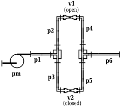
For clarity purposes, the hydraulic system depicted in Figure 1, called System A, will be used as an example throughout the paper. It is composed by a volumetric pump ✵ ✕ , pipes ✵ ✷ , ✵ ✹ , ✵ ✻ , ✵ ✽ , ✵ ✾ , ✵ ✿ , and valves ❀ ✷ (in closed state) and ❀ ✹ (in open state). In Table 1, we define the component modes in System A (the formulae that specify the types of components and the connections among them can be easily derived from the schema in Figure 1). In the volumetric pump's behavioral description, ❃ ❄ , which depends on the pump's settings, is the amount of flow the normal pump is able to impose. To avoid unnecessary complex examples, we consider only flow observations.
| type | behavioral modes |
|---|---|
| ❆ ❇ ❉ ❆ | ❋ ● ■ ❏ ❆ ❇ ❉ ❆ ❋ ■ ❏ ◆ ❖ ❄ ❋ ■ ❏ ❘ ❙ ❚ ❯ ❱ ❖ ❲ ❋ ■ ❏ ❨ ❖ ❇ ❬ ❯ ❱ ❖ ❲ ❋ ■ ❏ ❨ ❭ ❫ ❋ ● ■ ❏ ❆ ❇ ❉ ❆ ❋ ■ ❏ ◆ ❱ ❵ ❛ ❄ ❋ ■ ❏ ❘ ❙ ❚ ❯ ❱ ❖ ❲ ❋ ■ ❏ ❝ ❖ ❇ ❬ ❯ ❱ ❖ ❲ ❋ ■ ❏ ❋ ● ■ ❏ ❆ ❇ ❉ ❆ ❋ ■ ❏ ◆ ❱ ❖ ❭ ❱ ❖ ❲ ❋ ■ ❏ ❘ ❙ ❚ ❯ ❱ ❖ ❲ ❋ ■ ❏ ❨ ❖ ❇ ❬ ❯ ❱ ❖ ❲ ❋ ■ ❏ ❢ ❭ ❫ ❋ ● ■ ❏ ❆ ❇ ❉ ❆ ❋ ■ ❏ ◆ ❣ ❙ ❭ ❱ ❖ ❲ ❋ ■ ❏ ❘ ❙ ❚ ❯ ❱ ❖ ❲ ❋ ■ ❏ ❨ ❖ ❇ ❬ ❯ ❱ ❖ ❲ ❋ ■ ❏ ❝ ❭ ❫ |
| ❆ ❙ ❆ ❵ | ❆ ❙ ❆ ❵ ❋ ■ ❏ ◆ ❚ ❖ ❦ ❉ ❛ ❱ ❋ ■ ❏ ❘ ❋ ❙ ❚ ❯ ❱ ❖ ❲ ❋ ■ ❏ ❨ ❖ ❇ ❬ ❯ ❱ ❖ ❲ ❋ ■ ❏ ❏ ❆ ❙ ❆ ❵ ❋ ■ ❏ ◆ ❱ ❵ ❛ ❄ ❋ ■ ❏ ❘ ❋ ❙ ❚ ❯ ❱ ❖ ❲ ❋ ■ ❏ ❝ ❖ ❇ ❬ ❯ ❱ ❖ ❲ ❋ ■ ❏ ❏ |
| ♠ ❛ ❱ ♠ ❵ | ♠ ❛ ❱ ♠ ❵ ❋ ■ ❏ ◆ ❖ ❆ ❵ ❚ ❋ ■ ❏ ◆ ❖ ❄ ❋ ■ ❏ ❘ ❋ ❙ ❚ ❯ ❱ ❖ ❲ ❋ ■ ❏ ❨ ❖ ❇ ❬ ❯ ❱ ❖ ❲ ❋ ■ ❏ ❏ ♠ ❛ ❱ ♠ ❵ ❋ ■ ❏ ◆ ✙ ❱ ❖ ♥ ❵ ♦ ❋ ■ ❏ ◆ ❖ ❄ ❋ ■ ❏ ❘ ❋ ❙ ❚ ❯ ❱ ❖ ❲ ❋ ■ ❏ ❨ ❖ ❇ ❬ ❯ ❱ ❖ ❲ ❋ ■ ❏ ❨ ♣ ❏ ♠ ❛ ❱ ♠ ❵ ❋ ■ ❏ ◆ ❱ ❵ ❛ ❄ ❋ ■ ❏ ❘ ❋ ❙ ❚ ❯ ❱ ❖ ❲ ❋ ■ ❏ ❝ ❖ ❇ ❬ ❯ ❱ ❖ ❲ ❋ ■ ❏ ❏ ♠ ❛ ❱ ♠ ❵ ❋ ■ ❏ ◆ ❖ ❆ ❵ ❚ ❋ ■ ❏ ◆ ♥ ❬ ❇ ✙ ❄ ✜ ❱ ❖ ♥ ❵ ♦ ❋ ■ ❏ ❘ ❋ ❖ ❇ ❬ ❯ ❱ ❖ ❲ ❋ ■ ❏ ❨ ♣ ❏ ♠ ❛ ❱ ♠ ❵ ❋ ■ ❏ ◆ ✙ ❱ ❖ ♥ ❵ ♦ ❋ ■ ❏ ◆ ♥ ❬ ❇ ✙ ❄ ✣ ❆ ❵ ❚ ❋ ■ ❏ ❘ ❋ ❖ ❇ ❬ ❯ ❱ ❖ ❲ ❋ ■ ❏ ❝ ♣ ❏ |
Structural abstraction decomposes a system into a hierarchy of subcomponents (or, vice versa, aggregates components into a hierarchy of supercomponents). We adopt the following terminology and assumptions. The structural abstraction of a diagnosis problem ✄ ❙ a114 ✆ ✝ ✄ ❙ a116 ✠ ✡ ✝ ❙ a116 ✌ ✠ ✎ ✏ ✝ ❙ ✓ 1 is a (more abstract) problem ✄ ❙ ✉ ✷ a114 ✆ ✝ ✄ ❙ ✉ ✷ , ✠ ✡ ✝ ❙ ✉ ✷ , ✌ ✠ ✎ ✏ ✝ ❙ ✉ ✷ ✓ , obtained by aggregating a subsystem (denoted by the set of components ✈ ✇ ✇ ② ③ ✌ ✠ ✎ ✏ ✝ ❙ ) into a single supercomponent ⑥ ✫ ⑦ ✌ ✠ ✎ ✏ ✝ ❙ ✉ ✷ .
The more abstract diagnosis problem ✄ ❙ ✉ ✷ represents the same system as ✄ ❙ , but: (i) from a structural point of view, the components belonging to ✈ ✇ ✇ ② have to be replaced by a single component ⑥ ✫ , and, (ii) from a behavioral point of view, a representation of the behavior of ⑥ ✫ has to be introduced. The behavior of ⑥ ✫ is reasonably a simplified representation of the possible combinations of behavioral modes of its subcomponents (e.g., by forgetting and/or collapsing some of the variables of components in ✈ ✇ ✇ ② ). Finally, also the set of observation ✠ ✡ ✝ ❙ ✉ ✷ could differ from ✠ ✡ ✝ ❙ , because observations that are internal to subsystem ✈ ✇ ✇ ② cannot be represented in ✄ ❙ ✉ ✷ . For example, suppose to aggregate pipe ✵ ✹ and open valve ❀ ✷ of System A into a component ⑥ ❶ ✷ of type ❀ ❷ ❸ ❀ ❶ , in open state. The choice is reasonable since when both ✵ ✹ and ❀ ✷ are normal, they act as an open valve, allowing fluid to flow. We can thus remove all the formulae which mention ✵ ✹ and ❀ ✷ , and introduce the theory ❹ ❀ ❷ ❸ ❀ ❶ ✆ ⑥ ❶ ✷ ✓ a116 ❼ ✵ ❶ ❽ ✆ ⑥ ❶ ✷ ✓ , ❼ ❾ ❿ ➀ ❸ ❼ ➁ ✆ ✵ ✷ ✓ a114
1 In this paper, we adopt the convention of using a greater subscript to indicate a more abstract, less complex theory.
➂ ❽ ➀ ❸ ❼ ➁ ✆ ⑥ ❶ ✷ ✓ ➃ ➂ ❽ ➀ ❸ ❼ ➁ ✆ ✵ ✻ ✓ , ❼ ❾ ❿ ➀ ❸ ❼ ➁ ✆ ⑥ ❶ ✷ ✓ a114 ➂ ❽ ➀ ❸ ❼ ➁ ✆ ✵ ✽ ✓ ➄ . In this case, the abstraction removes the flow measurement at the connection between ✵ ✹ and ❀ ✷ , and keeps the other measurements.
We define a hierarchical representation of a given diagnostic problem ✆ ✝ ✄ ♣ , ✠ ✡ ✝ ♣ , ✌ ✠ ✎ ✏ ✝ ♣ ✓ as a list of ✕ diagnostic problems ❹ ✆ ✝ ✄ ❙ , ✠ ✡ ✝ ❙ , ✌ ✠ ✎ ✏ ✝ ❙ ✓ ➄ ❉ with ➂ a114 ➅ a116 ➆ ➆ ➆ a116 ✕ ➇ ➉ where for every ➋ a114 ➅ a116 ➆ ➆ ➆ a116 ✕ ➇ ➌ , ✄ ➎ ✉ ✷ is a structural abstraction of ✄ ➎ . A possible 6-levels hierarchical representation of System A is sketched in Table 2. Each row of the table shows a level of the hierarchical representation. For each level, we indicate the level number, the components (together with their type), and the aggregations performed to obtain that level (in the third column of the table, ✫ ❙ + ✫ ➎ ➐ ⑥ ✫ means that ✫ ❙ and ✫ ➎ have been aggregated into ⑥ ✫ ).
In order to ensure correctness and completeness when reasoning with abstract system representations, structural abstractions must satisfy some constraints. More specifically, the following property must be satisfied.
Property 1 (Relation between diagnoses). Let ✄ ❙ a116 ✄ ❙ ✉ ✷ be diagnosis problems, such that ✄ ❙ ✉ ✷ is a structural abstraction of ✄ ❙ . Let ✰ and ➑ be candidates of ✄ ❙ and ✄ ❙ ✉ ✷ , respectively, and suppose that ➑ is a more abstract representation of ✰ (according to the aggregation that has been performed in order to obtain ✄ ❙ ✉ ✷ ). If ➑ is not a diagnosis of ✄ ❙ ✉ ✷ , then ✰ must not be a diagnosis of ✄ ❙ .
If this property is satisfied, one can rule out candidates at the more detailed level by reasoning only at the abstract level, because structural abstraction never mistakenly rules out a diagnosis. On the negative side, diagnosis must consider also the more detailed level in order to ensure correctness and completeness of results. We now show that similar requirements are imposed by other formalizations of structural abstraction proposed in the literature. Thus, the techniques we present are not constrained to a specific formalization. In the following, let ✫ ✷ a116 ➆ ➆ ➆ a116 ✫ ❄ be a set of components which is aggregated into the supercomponent ⑥ ✫ , and ❼ ➒ ✆ ✫ ✓ a formula saying that component ✫ is behaving normally.
In [Struss, 1992], structural abstraction is defined as follows. Supercomponent ⑥ ✫ is a structural abstraction of ✫ ✷ a116 ➆ ➆ ➆ a116 ✫ ❄ if ❼ ➒ ✆ ✫ ✷ ✓ ➓ ➔ ➔ ➔ ➓ ❼ ➒ ✆ ✫ ❄ ✓ ➣ ❼ ➒ ✆ ⑥ ✫ ✓ . In this way, whenever ❼ ➒ ✆ ⑥ ✫ ✓ is inconsistent with the observations, then also ❼ ➒ ✆ ✫ ✷ ✓ ➓ ➔ ➔ ➔ ➓ ❼ ➒ ✆ ✫ ❄ ✓ is inconsistent, i.e. by excluding at the abstract level that ⑥ ✫ is normal, we can exclude also that all its subcomponents are normal. This is a special case of Property 1 when we represent only the normal behavior of components in ✝ ✄ .
[Mozetic, 1992] (using a different formalization of diagnosis) lists a set of consistency conditions that must hold between a system representation and its more abstract version. These conditions ensure that Property 1 holds.
[Autio and Reiter, 1998] formalizes structural abstraction for diagnosis problems where only the correct behavior of components is represented. Their approach requires both that ❼ ➒ ✆ ✫ ✷ ✓ ➓ ➔ ➔ ➔ ➓ ❼ ➒ ✆ ✫ ❄ ✓ ➣ ❼ ➒ ✆ ⑥ ✫ ✓ (as in Struss' formalization) and that ❼ ➒ ✆ ⑥ ✫ ✓ ➣ ❼ ➒ ✆ ✫ ✷ ✓ ➓ ➔ ➔ ➔ ➓ ❼ ➒ ✆ ✫ ❄ ✓ (i.e., if ⑥ ✫ is behaving normally, we can conclude that all its subcomponents are behaving normally). The second assumption can cause incorrect diagnoses when structural abstraction hides some measurements ➛ (e.g. there is a sensor which is "hidden" inside ⑥ ✫ ). Indeed, because of the lacking measurement, one could conclude that the normal behavior of ⑥ ✫ is consistent with the observations, and thus infer that all ⑥ ✫ 's subcomponents are also behaving normally, which in general is not true.
3 Analysis of Mozetic's approach
We illustrate Mozetic's diagnostic algorithm in a format that will allow us to easily compare it with our proposal and highlight the refinements we made. The inputs of the algorithm are the hierarchical representation, and a set ✠ ✡ ✝ ♣ of observations at the finest level of detail (i.e., level ➅ ). For each level ➂ of the hierarchical representation, ✌ ❷ ❽ ➜ ➝ ➞ ❙ is the set of candidates which have no abstraction at upper levels. Hierarchical diagnosis is formalized as follows:
Procedure HIERARCHICAL-DIAGNOSIS ABSTRACT-OBSERVATIONS; TOP-DOWN-DIAGNOSIS.Procedure ABSTRACT-OBSERVATIONS ➠ ➡ ➤ ; ➦ ➡ number of levels of the hierarchical representation; WHILE ➠ ➧ ➦ ➨ ➩ ➭ ➯ ➲ ➵ ➸ ➺ ➻ ➼ DO ➯ ➲ ➵ ➸ ➾ ➚ ➡ Abstract( ➯ ➲ ➵ ➸ ); ➠ ➡ ➠ ➶ ➩ ; ENDWHILE; IF ➯ ➲ ➵ ➸ ➻ ➼ THEN ➠ ➡ ➠ ➨ ➩ ➹ Procedure TOP-DOWN-DIAGNOSIS ➘ ➴ ➷ ➡ ➠ ; ➬ ➮ ✃ ❐ ➸ ➡ all possible candidates at level ➠ ; WHILE ➠ ❒ ➤ DO ❰ a207 ➮ a208 ➸ ➡ Verify( ➵ ❰ ➸ a209 ➯ ➲ ➵ ➸ a209 ➬ ➯ a210 a211 ➵ ➸ a209 ➬ ➮ ✃ ❐ ➸ ); IF ➠ ➧ ➘ ➴ ➷ THEN ❰ a207 ➮ a208 a212 a213 ➸ ➡ Verifya214 ➵ ❰ ➸ a209 ➯ ➲ ➵ ➸ a209 ➬ ➯ a210 a211 ➵ ➸ a209 ➬ ➮ ✃ ❐ a212 a213 ➸ ); ❰ a207 ➮ a208 ➸ ➡ ❰ a207 ➮ a208 ➸ a215 ❰ a207 ➮ a208 a212 a213 ➸ ; ENDIF; IF ➠ a216 ➤ THEN ➬ ➮ ✃ ❐ ➸ a217 ➚ ➡ Detailed( ❰ a207 ➮ a208 ➸ ); ➠ ➡ ➠ ➨ ➩ ;ENDWHILE.
| level | components | aggregations |
|---|---|---|
| ✾ | ❆ ❇ ❉ ❆ ❋ ♥ ❵ a218 ❏ | ♥ ❵ a219 ✉ ♥ ❵ a220 a221 ♥ ❵ a218 |
| ✽ | ❆ ❇ ❉ ❆ ❋ ♥ ❵ a220 ❏ a222 ♠ ❛ ❱ ♠ ❵ ❋ ♥ ❵ a219 ❏ | ❆ ❉ ✉ ❆ a223 a221 ♥ ❵ a219 a222 ❆ ❛ a223 ✉ ❆ a220 a221 ♥ ❵ a220 |
| ✻ | ❆ ❇ ❉ ❆ ❋ ❆ ❉ ❏ a222 ❆ ❙ ❆ ❵ ❋ ❆ a223 ❏ a222 ❆ ❙ ❆ ❵ ❋ ❆ a220 ❏ a222 ♠ ❛ ❱ ♠ ❵ ❋ ❆ ❛ a223 ❏ | ♥ ❵ a224 ✉ ♥ ❵ a225 a221 ❆ ❛ a223 |
| ✹ | ❆ ❇ ❉ ❆ ❋ ❆ ❉ ❏ a222 ❆ ❙ ❆ ❵ ❋ ❆ a223 ❏ a222 ❆ ❙ ❆ ❵ ❋ ❆ a220 ❏ a222 ♠ ❛ ❱ ♠ ❵ ❋ ♥ ❵ a224 ❏ a222 ♠ ❛ ❱ ♠ ❵ ❋ ♥ ❵ a225 ❏ | ♥ ❵ a223 ✉ ❆ a225 a221 ♥ ❵ a224 a222 ♥ ❵ a227 ✉ ❆ a219 a221 ♥ ❵ a225 |
| ✷ | ❆ ❇ ❉ ❆ ❋ ❆ ❉ ❏ a222 ❆ ❙ ❆ ❵ ❋ ❆ a223 ❏ a222 ❆ ❙ ❆ ❵ ❋ ❆ a220 ❏ a222 ♠ ❛ ❱ ♠ ❵ ❋ ♥ ❵ a223 ❏ a222 ❆ ❙ ❆ ❵ ❋ ❆ a219 ❏ a222 ♠ ❛ ❱ ♠ ❵ ❋ ♥ ❵ a227 ❏ a222 ❆ ❙ ❆ ❵ ❋ ❆ a225 ❏ | ❆ a227 ✉ ♠ a223 a221 ♥ ❵ a223 a222 ❆ a224 ✉ ♠ a227 a221 ♥ ❵ a227 |
| ♣ | ❆ ❇ ❉ ❆ ❋ ❆ ❉ ❏ a222 ❆ ❙ ❆ ❵ ❋ ❆ a223 ❏ a222 ❆ ❙ ❆ ❵ ❋ ❆ a220 ❏ a222 ♠ ❛ ❱ ♠ ❵ ❋ ♠ a223 ❏ a222 ❆ ❙ ❆ ❵ ❋ ❆ a224 ❏ a222 ❆ ❙ ❆ ❵ ❋ ❆ a219 ❏ a222 ♠ ❛ ❱ ♠ ❵ ❋ ♠ a227 ❏ a222 ❆ ❙ ❆ ❵ ❋ ❆ a227 ❏ a222 ❆ ❙ ❆ ❵ ❋ ❆ a225 ❏ |
Table 2: Components in the hierarchical representation for system A.
cedures. The first one (ABSTRACT-OBSERVATIONS) associates the available observations to the abstract levels of the hierarchical representation. Then, the second one (TOPDOWN-DIAGNOSIS) performs the diagnosis.
In particular, ABSTRACT-OBSERVATIONS takes as input the initially available observations ✠ ✡ ✝ ♣ , and, by repeatedly applying the Abstract function (corresponding to the abstract predicate in Mozetic's original formulation), determines the available observations (if any) for the more abstract levels. The number associated to the coarsest level with observations available is then stored into variable ❸ . The levels from ❸ to ➅ are then considered by the procedure TOPDOWN-DIAGNOSIS: for each level ➂ , first diagnosis is performed using the Verify function (corresponding to Mozetic's verify predicate); then, the diagnoses that are found are translated into their representations at the next more detailed level by the function Detailed (corresponding to Mozetic's detailed predicate). Those diagnoses will be the possible candidates for level ➂ ➇ ➉ . Moreover, also those candidates (if they exist) which have no abstraction at upper levels, and are thus considered for the first time at the current level, are verified. When level 0 is reached, the final diagnoses are returned. It must be noted that no assumptions are made on the implementation of the Verify function (e.g. it can be a generate-andtest method, a GDE-like reasoner, or other MBD technique).
By performing diagnosis at more abstract levels, Mozetic aims at finding those diagnoses that are impossible, thus reducing the number of possible diagnoses, i.e. the size of the search space, at more detailed levels. This makes it possible, in many cases, to perform significantly better than directly solving the most detailed diagnosis problem. Experiments done by Mozetic report, in a medical example using a fourlevel qualitative model of the heart, a speed up by a factor of 20 over a one-level diagnosis. However, given a hierarchical representation, there are situations where the performance is not as good as one would expect because only part of the hierarchical representation is exploited, as we show in the following.
Example 1. Consider the 6-levels hierarchical representation of System A sketched in Table 2, and suppose that the following observations are available: flow at the input of pipe ✵ ✹ is ❷ a229 ❃ ❄ , while flow at the output of valve ❀ ✷ is a231 a232 ❃ ❄ , i.e. ✠ ✡ ✝ ♣ a114 ❹ ➂ ❽ ➀ ❸ ❼ ➁ ✆ ✵ ✹ ✓ a114 ❷ ➓ ❼ ❾ ❿ ➀ ❸ ❼ ➁ ✆ ❀ ✷ ✓ a114 a231 ➄ . Executing ABSTRACT-OBSERVATIONS, the observation at the input of ✵ ✹ can be abstracted to level 1 as the input of ⑥ ❶ ✷ , but cannot be abstracted to level 2, where the input of ✵ ✹ is not visible anymore. By applying the same line of reasoning, the observation on ❀ ✷ is abstracted up to level 2. The TOPDOWN-DIAGNOSIS procedure can thus start only at level 2.
In this example, diagnostic reasoning considers only the three more detailed levels of the hierarchical representation (no observations can be abstracted higher than level 3), and thus cannot take any advantage from the remaining coarser levels, where reductions of the search space could be in principle obtained with less effort. The result is that the computational savings gained over a plain, one-level diagnosis are not as good as one would expect, because diagnosis is started at an intermediate level of the hierarchy.
In general, when we structurally abstract a diagnosis problem, all the observations that refer only to components that are aggregated become unavailable. Thus, as we climb the hierarchical representation, less observations are available. In the systems where the position of measurement sensors is known and cannot be changed, one can limit this problem by choosing the aggregations in such a way that the most abstract levels have always (or at least often) some observation available. However, in general, whatever hierarchical representation we exploit, as the total number of given observations decreases, the top level from which diagnosis is started tends to become lower, i.e. the number of abstract levels not considered for diagnosis increases. The worst consequence of this problem is that the performance of Mozetic's algorithm can become identical to a plain diagnostic approach. This happens whenever the observations given as input cannot be abstracted to level 1, i.e. when all observations refer only to components that are aggregated in order to obtain level 1. The following example shows one possible scenario in which this situation occurs in System A.
Example 2. Suppose that the following observations are available: flow at the output of pipe ✵ ✻ is ❷ a229 ➅ , i.e. ✠ ✡ ✝ ♣ a114 ❹ ❼ ❾ ❿ ➀ ❸ ❼ ➁ ✆ ✵ ✻ ✓ a114 ❷ ➄ . The observation on the output of ✵ ✻ cannot be abstracted to level 1, because it is not present at that level. Hence, at the end of the execution of the ABSTRACTOBSERVATIONS procedure, the most abstract level with observations is level 0. Thus, diagnosis is started at that level.
4 Our proposed approach
We propose a technique that aims at improving Mozetic's strategy when structural abstractions are used. Our approach exploits also an additional data structure, called structural tree (presented in Section 4.1), that highlights the aggregations performed to build the hierarchical representation.
4.1 The structural tree
We associate any hierarchical representation a234 (built with structural abstractions) to a Structural Tree for a234 called ST(H). In the tree, each node represents a component of a234 , and its sons are its subcomponents.
Given a hierarchical representation of a diagnostic problem a234 a114 ❹ ✆ ✝ ✄ ❙ , ✠ ✡ ✝ ❙ , ✌ ✠ ✎ ✏ ✝ ❙ ✓ ➄ ❉ a116 ➂ a114 ➅ a116 ➆ ➆ ➆ a116 ✕ ➇ ➉ , ST(H) is built as follows:
- a235 first, for each component ➀ ⑦ ✌ ✠ ✎ ✏ ✝ ♣ , a new leaf ➀ is created;
- a235 then, for each aggregation of ✫ ✷ a116 ➆ ➆ ➆ ✫ ❄ ⑦ ✌ ✠ ✎ ✏ ✝ ❙ into ⑥ ✫ ⑦ ✌ ✠ ✎ ✏ ✝ ❙ ✉ ✷ such that ✫ ✷ a116 ➆ ➆ ➆ ✫ ❄ ⑦ ✝ a238 ✆ a234 ✓ , a new node ⑥ ✫ is created such that ⑥ ❼ ❽ ⑥ ✆ ⑥ ✫ ✓ a114 ✫ ✷ a116 ➆ ➆ ➆ a116 ✫ ❄ .
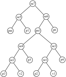
The root of ✝ a238 ✆ a234 ✓ is associated with the component that represents the whole system, i.e. a239 ❼ ❼ ❿ ✆ ✝ a238 ✆ a234 ✓ ✓ a114 ✫ ⑦ ✌ ✠ ✎ ✏ ✝ ❉ a240 ✷ . Figure 2 shows the structural tree for System A which has been obtained from the 6-level hierarchical representation sketched in Table 2.
Since each node ✫ of ST(H) is a component ✫ ⑦ ✌ ✠ ✎ ✏ ✝ ❙ for some ➂ , we associate to it the theory ✝ ✄ ✙ ③ ✝ ✄ ❙ and the observations ✠ ✡ ✝ ✙ ③ ✠ ✡ ✝ ❙ (when they are available). Thus, each node ✫ is associated with a subset of one of the diagnostic problems of a234 .
4.2 The Rearrange algorithm
We propose a technique that dynamically determines a new hierarchical representation suited to diagnose the specific situation described by the current observations. The new hierarchical representation will be built by rearranging the levels of a given hierarchical representation a234 using the corresponding ST(H) on the basis of the available observations.
The idea is to improve Mozetic's algorithm when it is not able to fully exploit the hierarchical representation, by providing a new, tailored hierarchical representation consisting of: (i) all levels of the original hierarchical representation which have observations (i.e. the levels considered by Mozetic's algorithm), and (ii) additional, more abstract levels which are not present in the original hierarchy, and have the same observations of the coarsest level considered by Mozetic's algorithm.
We will now show, using an example, how these additional levels can be built with little effort. In some cases, indeed, the abstract level at which diagnosis is started by Mozetic's algorithm is too detailed than necessary. Consider the scenario presented in Example 2, where diagnosis is started at level 0 (which contains 9 components), without exploiting the possibility of starting from a more abstract diagnosis problem. For example, the diagnosis problem (let us call it Best) with components ⑥ ❶ ✾ , ⑥ ❶ ✻ , ✵ ✻ , ❀ ✹ , ✵ ✾ , and ✵ ✿ is more abstract than level 0 but has the same observations (i.e. ❼ ❾ ❿ ➀ ❸ ❼ ➁ ✆ ✵ ✻ ✓ a114 ❷ ). The search space of Best is much smaller: the diagnosis problem at level 0 has 2304 possible candidates, while ✡ ❶ ⑥ ❿ has 288 possible candidates.
Mozetic's algorithm cannot start from ✡ ❶ ⑥ ❿ because this diagnosis problem is not available in the given hierarchical representation: the only level with observations is level 0. The problem is that the algorithm exploits the representation in a "fixed" way: levels are identical for any set of observations, and only the choice of starting level changes.
We can derive ✡ ❶ ⑥ ❿ by selecting nodes in the structural tree of Figure 2. The structural tree highlights indeed the aggregations used in a hierarchical representation, regardless of the order in which they were performed. One can derive ✡ ❶ ⑥ ❿ by selecting a set of nodes in the structural tree which: (i) represent the full system, (ii) have the same observations that are present at level where Mozetic's algorithm starts, (iii) are as abstract as possible. Then, one can compose the theories associated to the selected nodes to derive a new, more abstract starting ✩ level.
We implemented this strategy as an extension to Mozetic's algorithm, which we call the REARRANGE extension. More specifically, the building of the new levels is performed as an additional activity after the ABSTRACT-OBSERVATION procedure, as shown in the following:
Procedure HIERARCHICAL-DIAGNOSIS
ABSTRACT-OBSERVATIONS;
REARRANGE;
TOP-DOWN-DIAGNOSIS.
Procedure REARRANGE IF ➠ ➧ ➦ ➨ ➩ THEN FOR each node ✃ of ➵ ✪ a214 ✬ ✮ referred in ➯ ➲ ➵ ➸ ➴ ✰ ✲ ✴ ➡ ✶ ➮ ➻ ✸ ✺ ➮ ➻ ✸ ✽ ➯ ➲ ➵ ➸ ➭ ➮ is a port of ✃ ✿ ; ❀ ➴ ❐ ❁ ✲ ❃ ❅ ➡ ➬ ➯ a210 a211 ➵ ➸ ; WHILE ❀ ➴ ❐ ❁ ✲ ❃ ❅ ➺ ➻ ➼ DO ✃ ➡ ❈ a207 ❊ ✲ ➘ a214 ❀ ➴ ❐ ❁ ✲ ❃ ❅ ✮ ; ❈ ➡ ❈ ➮ ➘ ● ❁ ❊ a214 ✃ ✮ ; IF ✲ ➴ ✃ ✲ a214 ❈ ✮ ■ ➬ ➯ a210 a211 ➵ ➸ ➭ a214 ❑ ▼ ❖ ▼ ❘ ✴ ▼ ❚ ❯ ❲ ➴ ✰ ✲ ▼ ✮ ➻ ➴ ✰ ✲ ❯ THEN ❀ ➴ ❐ ❁ ✲ ❃ ❅ ➡ a214 ❀ ➴ ❐ ❁ ✲ ❃ ❅ ➨ ✲ ➴ ✃ ✲ a214 ❈ ✮ ✮ a215 ✶ ❈ ✿ ; ➠ ➡ ➠ ➶ ➩ ; ➬ ➯ a210 a211 ➵ ➸ ➻ a214 ➬ ➯ a210 a211 ➵ ➸ a217 ➚ ➨ ✲ ➴ ✃ ✲ a214 ❈ ✮ ✮ a215 ✶ ❈ ✿ ; ADD a new level numbered ➠ with components ➬ ➯ a210 a211 ➵ ➸ to the hierarchical representation ✬ ; ❀ ➴ ❐ ❁ ✲ ❃ ❅ ➡ ➬ ➯ a210 a211 ➵ ➸ ; ELSE ❀ ➴ ❐ ❁ ✲ ❃ ❅ ➡ ❀ ➴ ❐ ❁ ✲ ❃ ❅ ➨ ✲ ➴ ✃ ✲ a214 ❈ ✮ ; ENDIF; ENDWHILE; ENDIF.The new activities performed by the procedure are:
- a235 each observation available at Mozetic's coarsest level with observations is associated to the corresponding nodes in ST(H) (obtaining the ❼ a231 ⑥ ❚ sets);
- a235 if possible, new diagnosis problems, which are more abstract than the one at which Mozetic starts, are added to a234 . These new levels are built by:
- considering the components of the current, most abstract level (which initially is the original coarsest level with observations);
- finding a subset of components that are all the sons of a node ➀ in ✝ a238 ✆ a234 ✓ such that the union of the observations associated to them are exactly the observations associated to ➀ (i.e. by substituting them with their father we do not hide any observation);
- if such set of components does exist, adding to a234 a new level whose components are the components of the current level which are not sons of ➀ , and ➀ itself. In this way, we build a more abstract diagnosis problem without losing any observation;
- if such set of components does not exist, the algorithm stops; otherwise, the search for components which meet the above described requirements is repeated considering the components of the newly derived level.
After the execution of REARRANGE, ❸ is the number of the new top level from which diagnosis is started. Note that, given the currently available observations, if ABSTRACTOBSERVATIONS is able to reach the most abstract level, then REARRANGE does nothing, and the whole reasoning proceeds exactly as in Mozetic's algorithm. In order to show the advantages of this strategy with respect to Mozetic's algorithm, we will now reconsider the previously illustrated examples.
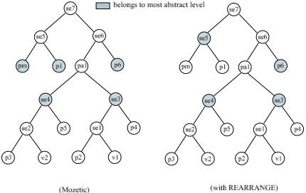
Example 3. Given the observations in Example 1, Mozetic's hierarchical diagnosis would start at level 2, which contains components ✵ ✕ , ✵ ✷ , ⑥ ❶ ✻ , ⑥ ❶ ✽ , and ✵ ✿ (see Figure 3, left). REARRANGE derives an additional, more abstract level 3. It contains components ⑥ ❶ ✾ , ⑥ ❶ ✻ , ⑥ ❶ ✽ , and ✵ ✿ (see Figure 3, right): components ✵ ✕ and ✵ ✷ of Mozetic's most abstract level with observations are aggregated into pump ⑥ ❶ ✾ . This is possible because ✵ ✕ and ✵ ✷ are the sons of ⑥ ❶ ✾ in the corresponding structural tree (that is, an aggregation for them is available), and the observations associated to them are the same associated to their father (in this case, ✵ ✕ , ✵ ✷ , and ⑥ ❶ ✾ have no observations). No coarser level can be derived, because there is no node in the structural tree whose sons belong to the newly derived level 3 and that can be aggregated without losing observations. Thus, REARRANGE stops. TOPDOWN-DIAGNOSIS starts from the newly derived level 3.
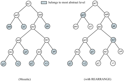
Example 4. The observations given in Example 2 cannot be abstracted to level 1. Hence, the most abstract level with observations is level 0. By applying our technique, first a new level is derived with components ✵ ✕ , ✵ ✷ , ✵ ✻ , ⑥ ❶ ✷ , ❀ ✹ , ✵ ✽ , ✵ ✾ , and ✵ ✿ (✵ ✹ and ❀ ✷ can be aggregated without eliminating observations); then, an additional level is derived with components ✵ ✕ , ✵ ✷ , ⑥ ❶ ✻ , ✵ ✻ , ❀ ✹ , ✵ ✾ , and ✵ ✿ ( ⑥ ❶ ✷ and ✵ ✽ can be aggregated without losing observations); finally, a most abstract level (from which diagnosis will start) is derived with components ⑥ ❶ ✾ , ⑥ ❶ ✻ , ✵ ✻ , ❀ ✹ , ✵ ✾ and ✵ ✿ (✵ ✕ and ✵ ✷ can be aggregated without losing observations). The most abstract level used by Mozetic and by our algorithm are graphically illustrated in Figure 4.
5 Experimental Evaluation
We experimentally evaluated our extension with respect to the original Mozetic's algorithm. Both algorithms were implemented in SWI Prolog (ISO-compliant free source Prolog) developed by the University of Amsterdam and run on a PowerPC G3 400 Mhz (Apple iMac DV) under the LinuxPPC 2000 operating system. The Verify procedure used by both algorithms was implemented as a generate-and-test algorithm, i.e. a procedure that considers each possible candidate and then verifies its consistency with the system description and observations. Obviously, this is the worst choice for implementing the Verify procedure, but it gives us a worst case scenario (corresponding to the exact size of the considered portion of the search space).
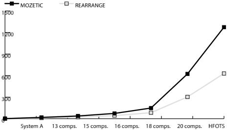
The experimental comparison was performed with diagnosis problems of different size in the hydraulic domain. The considered systems differed in the layout and in the number of components and ports. More precisely, the simplest considered system was System A (9 components), and the most complex was an Heavy Fuel Oil Transfer System (27 components) of a container ship. For each hydraulic system, we considered several possible sets of observations. Each set contained a number of observations randomly selected between one and ❩ ❖ ❬ ♥ , with ❩ ❖ ❬ ♥ a114 ❿ a239 ❾ ❽ ✫ ✆ ➅ ➆ ❪ ❫ ❽ ✓ where ❽ is the number of possible measurements points for the considered system (e.g. in systems with 10 possible measurement points, each set contained between one and four observations). The justification for this choice is twofold: first, with a few observations, the problem is more difficult (and this is the typical case in which one wants to use abstraction); second, in the majority of real cases, observations are very scarce because of cost and reliability of sensors, so considering more observations is not a realistic scenario. Each set with ➒ observations was generated by assigning a random value to ➒ measurements points (randomly selected between the available ones). Figure 5 illustrates the average CPU times we obtained with the considered hydraulic systems considering 1000 different sets of observations for each system. As one can see, for both algorithms the average CPU time becomes very high for small increases of the number of components of the considered systems (this is due to the generate-and-test procedure). However, our extension performs significantly better, and is more effective as the size of the considered system increases. This is due to the fact that, in a hierarchical representation with many components and levels, REARRANGE has more opportunities for deriving additional levels, and thus obtaining greater improvements. Finally, the experimental evaluation shows that the advantages REARRANGE brings to hierarchical diagnosis outperform the cost of its additional activities.
6 Conclusions
We presented an extension to Mozetic's algorithm that improves its performance when structural abstractions are employed. Although improvements were demonstrated experimentally, we definitively need to test our approach with other real-world systems in different domains to evaluate its effectiveness. Moreover, we are also working on alternative rearrangements of hierarchical representations which can be more effective in some situations. Finally, we are considering to include the cost and discrimination power of measurements in the rearrangement process.
@inproceedings{ijcai2001p80,
  title     = {Hierarchical Diagnosis Guided by Observations},
  author    = {Chittaro, Luca and Ranon, Roberto},
  booktitle = {Proceedings of the Seventeenth International Joint Conference on
               Artificial Intelligence, {IJCAI-01}},
  publisher = {International Joint Conferences on Artificial Intelligence},
  editor    = {Bernhard Nebel},
  pages     = {573--577},
  year      = {2001},
  url       = {https://ijcai.org/proceedings/2001/80},
}
TY - CPAPER TI - Hierarchical Diagnosis Guided by Observations AU - Chittaro, Luca AU - Ranon, Roberto T2 - Proceedings of the Seventeenth International Joint Conference on Artificial Intelligence, IJCAI-01 PB - International Joint Conferences on Artificial Intelligence PY - 2001 SP - 573 EP - 577 UR - https://ijcai.org/proceedings/2001/80 ER -Copied
Machine-readable versions of this paper, for tools and AI agents:





