
Coupling CSP Decomposition Methods and Diagnosis Algorithms for Tree-Structured Systems
Proceedings of the Eighteenth International Joint Conference on Artificial Intelligence. Pages 388-392.
© 2003 International Joint Conferences on Artificial Intelligence
Abstract
Decomposition methods are used to convert general constraint satisfaction problems into an equivalent tree-structured problem that can be solved more effectively. Recently, diagnosis algorithms for treestructured systems have been introduced, but the prerequisites of coupling these algorithms to the outcome of decomposition methods have not been analyzed in detail, thus limiting their diagnostic applicability. In this paper we generalize the TREE* algorithm and show how to use hypertree decomposition outcomes as input to the algorithm to compute the diagnoses of a general diagnosis problem.
- [Darwiche, 1998] Adnan Darwiche. Compiling Devices: A Structure-Based Approach. In Proceedings of the Interna- tional Conference on Principles of Knowledge Represen- tation and Reasoning, pages 156-166, 1998.
- [de Kleer and Williams, 1987] Johan de Kleer and Brian C. Williams. Diagnosing multiple faults. Artificial Intelli- gence, 32(1):97-130, 1987.
- [de Kleer, 1991] Johan de Kleer. Focusing on probable di- agnoses. In Proceedings of the National Conference on Artificial Intelligence (AAAI), pages 842-848, Anaheim, July 1991.
- [Dechter and Pearl, 1989] Rina Dechter and Judea Pearl. Tree clustering for constraint networks. Artificial Intel- ligence, 38 :353-366, 1989.
- [Fattah and Dechter, 1995] Yousri El Fattah and Rina Dechter. Diagnosing tree-decomposable circuits. In Proceedings 14th International Joint Conf on Artificial Intelligence, pages 1742-1748, 1995. IJCAI
- [Freuder, 1985] Eugene C. Freuder. A Sufficient Condition for Backtrack-Bounded Search. Artificial Intelligence, 32(4):755-761, 1985.
- [Gottlob eta/., 1999a] Georg Gottlob, Nicola Leone, and Francesco Scarcello. Hypertree Decomposition and Tractable Queries. In Proc. 18th ACM SIGACT SIGMOD SIGART Symposium on Principles of Database Systems (PODS-99), pages 21-32, Philadelphia, PA, 1999.
- [Gottlob eta/., 1999b] Georg Gottlob, Nicola Leone, and Francesco Scarcello. On Tractable Queries and Con- straints. In Proc. I 2th International Conference on Database and Expert Systems Applications DEXA 2001, Florence, Italy, 1999.
- [Gottlob eta/., 2000] Georg Gottlob, Nicola Leone, and Francesco Scarcello. A comparison of structural CSP de- composition methods. Artificial Intelligence, 124(2):243- 282, December 2000. IJCAI
- [Gottlob et al. , 2002] Georg Gottlob, Martin Hutle, and Franz Wotawa. Combining hypertree, bicomp, and hinge decomposition. In F. van Harmelen, editor, Proceedings of the 15th European Conference on Artificial Intelligence (ECAI-02), Lyon, July 2002. lOS Press.
- [Gyssens et al., 1994] Marc Gyssens, Peter G. Jeavons, and David A. Cohen. Decomposing constraint satisfaction problems using database techniques. Artificial Intelli- gence, 66:57-89, 1994.
- [Mauss and Tatar, 2002] Jakob Mauss and Mugur Tatar. Computing minimal conflicts for rich constraint lan- guages. In F. van Harmelen, editor, Proc. ECAI, Ams- terdam, 2002. lOS Press.
- [Reiter, 1987] Raymond Reiter. A theory of diagnosis from first principles. Artificial Intelligence, 32(1):57-95, 1987.
- [Stumptner and Wotawa, 2001] Markus Stumptner and Franz Wotawa. Diagnosing tree-structured systems. Artificial Intelligence, 127(1): 1-29,2001. IJCAI
References were extracted automatically from the PDF and may contain errors.
Full text extracted automatically from the PDF; figures, tables and equations may differ. The PDF is the version of record.
1 Introduction
The development of effective algorithms for diagnosing large and complex systems remains one of the key issues in model based reasoning. Nonetheless, apart from various additional optimizations and control strategies (e.g., [de Kleer, 1991]) the main architectures for consistency-based diagnosis sys tems, TMS [de Kleer and Williams, 1987] and hitting sets computation [Reiter, 1987], have remained remarkably sta ble since the late 1980s. Over the last years though, a num ber of algorithms were published that exploited advantageous structural properties of the systems to be diagnosed for sig nificant computational speedups [Fattah and Dechter, 1995; Stumptner and Wotawa, 2001 ], enabling the very fast diagno sis of large tree-structured systems.
It was recognized early on that the combination of tree oriented algorithms could in principle be combined with a second class of algorithms aiming at the decomposition of cyclic problems to equivalent tree-structured problems so that the faster solution algorithms could be brought to bear [Fat tab andDechter, 1995; Darwiche, 1998]. Again, this direction profits from recent new results relating the different decom position algorithms [ Gottlob et a!., 2000] and analyzing their performance [Gottlob eta!., 2002]. This paper joins the two strands by tying the link between the recent work on prob lem decomposition and the TREE* algorithm [Stumptner and Wotawa, 200 1].
*This work was partially supported by the Austrian Science Fund (FWF) under project grants Pl5163-INF and Pl5265-INF.
t Authors are listed in alphabetical order.
Franz Wotawa t Technische Universitiit Graz Institute for Software Technology (IST) 8010 Graz, Inffeldgasse 16b/2, Austria
wotawa@ist.tugraz.at
This combination is aided by the fact that both subar eas tend to use Constraint Satisfaction Problems (CSPs) as their representation of choice. The diagnosis computation work [Fattah and Dechter, 1995; Stumptner and Wotawa, 2001; Mauss and Tatar, 2002] focuses on the relational com bination of the different constraint relations, while the prob lem reformulation work views CSPs as (often cyclic) hyper graphs that are broken down into tree structures.
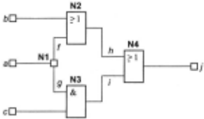
A CSP (V, D, C) comprises a set of variables V, their do mains D, and a set of constraints C. A constraint C i is tuple (S;, T;) where S; ~ Vis its scope and T; is a set of tuples of values for the variables inS;. We assume two functions tpl and scope on constraints that return the set of tuples and the scope respectively. Each constraint C i restricts the possible values of the variables with respect to values of other vari ables in the same scope.For example, the digital circuit from Figure 1 can be represented by the following constraints 1 :
| N1 | N2 | ||||
|---|---|---|---|---|---|
| a | f | g | f | b | h |
| 1 | 1 | 1 | 0 | 0 | 0 |
| 0 | 0 | 0 | 0 | 1 | 1 |
| 1 | 0 | 1 | |||
| 1 | 1 | 1 | |||
| N4 | |||||
| g | c | 1 | h | i | J |
| 0 | 0 | 0 | 0 | 0 | 0 |
| 0 | 1 | 0 | 0 | 1 | 1 |
| 1 | 0 | 0 | 1 | 0 | 1 |
| 1 | 1 | 1 | 1 | 1 | 1 |
A solution of a CSP is an assignment of values to all vari ables that satisfy the given constraints. All values must be elements of their variable's domain. The variable assignment b = l,a = O,c = O,J = O,g = O,h = 1,i = O,j = 1 is a solution for the above CSP whereas b = 1, a = 0, c = 0, f = 0, g = 0, h = 1, i = 0, j = 0 is not because constraint N4 is not satisfied.
A standard approach for computing solutions for CSPs are backtracking algorithms, which are in the worst case expo nential in the number of variables. However, for a specific class of CSPs a solution can be computed in polynomial time. This class comprises all CSPs that have an acyclic corre sponding hypergraph 2 · A hypergraph of a CSP can be eas ily construCted by mapping all variables of the CSP to ver tices and the constraint scopes to hyperedges. A CSP with an acyclic hypergraph can be solved effectively in a backtrack free manner by first traversing the graph from the leafs to the root and computing possible value tuples and secondly, traversing the graph from the root to the leafs and selecting one tuple of a node as a solution. The hypergraphcorrespond ing to Fig. 1 is cyclic (see Figure 2).
1 Note that not all constraints are components, N1 is the tabular representation of an equality constraint between connections).
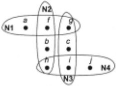
In the rest of the paper, we recapitulate decomposition methods, present a version of TREE* that fits these meth ods, show the interaction of decomposition and TREE*, and present an extension to the algorithm that can be used with extended domains as presented in [Mauss and Tatar, 2002].
2 Decomposition methods
Several different decomposition methods have been pub lished, most recently the hypertree decomposition method [Gottlob et a/., 1999a]. This and other structure-based de composition methods make compute a tree-structured sys tems from general CSPs by elimination of cycles from the CSP. A cycle can be eliminated by applying the relational al gebrajoin operation to the constraints on the cycle. However, blindly joining all constraints in the cycle can result in expo nential costs for computing the tuples of the joined constraint, and a key property of the different decomposition methods is the different techniques they use to select the constraints to be joined. Gottlob et al. [2000] compared different decompo sition methods with respect to their width, i.e., the maximum number of constraints to be joined, and found that hypertree decomposition is superior with respect to the width. Since hy pertree decomposition can be seen as a generalization of the other techniques, we restrict our examination here to hyper tree decomposition. Note that the result of a decomposition method is always a hypertree.
2 A hypergraph (N, E) consists of a set of vertices N and a set ofhyperedges E such that e ~ N for each e E E
In [ Gottlob et a/., 2000] hypertree decomposition is char acterized as follows. A hypertree of a hypergraph H is a triple (T, x, A) , where T = (N, E) is a rooted tree with vertices N and edges E, x and A are labeling functions which associate to each vertexp E N a set of variables A(p) ~ var(H) and a set of constraints x (p) ~ edges(H) . We further define x for a subtree T' = (N', E') ofT as x (T') = U vEN' x (v), and for any p E N, Tp denotes the subtree ofT rooted at p. We denote the root of a hypertree by root(T) .
Based on the above definitions, the hypertree decompo sition of a hypergraph H is defined as a hypertree H D = (T, x, A) where T = (N, E) which satisfies the following conditions:
- For each edge hE edges(H), there exists apE N such that var(h) ~ x (p) .
- For each variable Y E var(H) , the set {p E N IY E x (p)} induces a connected subtree ofT.
- For each pEN, x (p) ~ var(A(p)) .
- For each pEN, var(A(p)) n x(Tp) ~ x (p).
Moreover, we say that h E edges(H) is strongly covered in H D if there exists a vertexp EN such that var(h) ~ x (p) and h E A(p) . A hypertree decomposition H D of a hyper graph H is a complete decomposition of H if every edge of H is strongly covered in H D . Note that it is always possible to make an incomplete decomposition complete by adding new vertices to the decomposition. Gottlob et al. [1999b] gave an algorithm for computing (complete) hypertree decomposi tions.
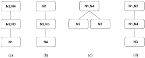
Note that unlike other decomposition methods such as bi connected component decomposition and hinge decomposi tion, there is in general no unique hypertree decomposition of a given CSP. Figure 3 shows four possible hypertree de compositions for the hypergraph depicted in Figure 2.
3 Diagnosis with TREE*
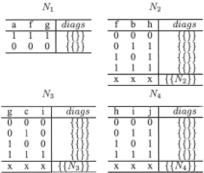
To be self contained we briefly recapitulate the TREE* algo rithm. Stumptner and Wotawa [2001] introduced the TREE* algorithm as an extension of the TREE algorithm. Both al gorithms work on tree-structured constraint systems. As op posed to TREE which requires the constraints to be mathe matical functions, TREE* imposes no limitations on the con straints. TREE* uses the following auxiliary functions asso ciated to constraints: constr denotes all tuples of the con straint. val denotes the tuples remaining after the application of TREE*. diags denotes the diagnoses that correspond to a given tuple. Accordingly, a CSP that is to be used for di agnosis purpose has to represent not only the tuples for each constraint but also the diagnoses that correspond to each tu ple. For example, the small circuit from Figure 1 can be rep resented by the following CSP:
| N1 | N2 | ||
|---|---|---|---|
| a f g diags 1 1 1 0 0 0 { {}} N3 | f b h 0 0 0 0 1 1 1 0 1 1 1 1 | diags | |
| g c i 0 0 | diags | X X X N4 h j 0 0 0 0 1 1 1 0 1 1 1 1 | diags |
| 0 0 1 0 1 0 0 1 1 1 X X X | X X X | ||
The tuples of form <x x ... x> in the above tables are in tended to match all tuples that are not explicitly given in the table. Note that the constraint N 1 represents a connection and is therefore assumed to be always correct. Hence, it always returns the empty set as a diagnosis.
The original description of the TREE* algorithm was based on the underlying assumption that the leaf vertices of the tree correspond only to one diagnosis component. This as sumption has an impact on the description of the algorithm, but not on the empirical results. If the constraints given to the algorithm do not satisfy this requirement, diagnoses of a size (i.e., number of faulty components) larger than specified might be returned because there is no way to remove these diagnoses from the set of tuples. The requirement did not constitute a hindrance since [Stumptner and Wotawa, 2001] did not deal with CSPs resulting from decomposition. To explicitly generalize TREE* to interact with decomposition algorithms, we here present a modified version that removes this requirement.
The following operations are used by TREE*: semi-join ( 1><) for constraints, Cartesian product ( x) for combining two sets of diagnoses, i.e., DS1 x DS2 = {d1 U d2ld1 E DS1 1\ d2 E DS2 }, and cardinality restriction (I) for remov ing diagnoses from a set of diagnoses with a size greater than the given value, i.e., DSis = {did E DS 1\ ldl <= s }.
Computes all diagnoses up to a pre-specified size for a given tree-structured diagnosis system.
Input: A decomposition H D with edges E, the root vertex p, and the pre-specified diagnosis size diagSize.
(1) V f- constr(p) 1>< observed(p) (2) for s E V do (3) diags(s) +- diags(s)ldiagSize (4) if diags(s) = 0 then (5) V+-V\{s} (6) end if (7) end for (8) for (p, q) E E do (9) TREE*(q) (10) V +- V 1>< val(q) (11) fors E V,t E val(q) suchthats,tjoindo (12) diags(s) f- (diags(s) x diags(t))ldiagSize (13) if diags(s) = 0 then (14) v f- v \ { s} (15) end if (16) end for (17) end forAlgorithm TREE* (H D, p, diagSize) Output: The diagnoses for each value tuple. (18) val(p) +- V
The TREE* algorithm is called using the rootp of the hy pertree, i.e., the result of a decomposition, as argument. After execution, the computed diagnoses can be found in the diag column of the tuples associated with the root p.
The TREE* algorithm correctly computes all diagnoses up to the given size if the following requirements are fulfilled:
- Every constraint is at least used in one of tree vertices.
- The induced subtree for every variable is connected.
Theorem 1 (Correctness) The TREE* algorithm correctly computes diagnoses up to the pre-specified size.
Proof. The proof is by induction over the size of the tree.
- Base step For each leaf of the tree only lines (l)-(7) and (18) of TREE* are executed. In these lines, all tu ples that contradict the given observations and all diag noses larger than the specified size are removed. Tuples with no corresponding diagnoses are removed. These steps do not prevent TREE* from computing a diagno sis. Hence, all diagnoses (up to the pre-specified size) are computed for leafs.
Hypothesis We assume that TREE* correctly computes di agnoses for trees of size smaller than n.
Induction step We now prove that TREE* correctly com putes the diagnoses for trees of size n. The steps ( 1 )-(7) only reduce the number of diagnoses. Tuples that con tradict the observations are removed. Diagnoses that are larger than the pre-specified values are removed and tu ples with a corresponding empty diagnosis set are also removed because they have no influence on the result. In step (9) the TREE* algorithm is called recursively. Be cause of our induction hypothesis, the algorithm returns correct diagnoses for each tuple. It remains to prove that the combination of these tuples with the tuple of the cur rent node is done correctly. Since every tuple that joins (line ( 11)) is considered and since that every diagnosis is combined with every diagnosis of the child vertices (line (12)), this process must lead to a correct result. Hence, TREE* correctly computes the diagnoses in step n as well. 0
Using the same arguments as above we can show that TREE* allows for computing all diagnoses providing that all the diagnoses for each vertex of the hypertree are computed. We omit the actual proof here.
Theorem 2 (Completeness) The TREE* algorithm com putes all diagnoses up to the pre-specified size.
The remaining issue now is to determine the conditions that a decomposition method must satisfy in order to be used with TREE*. Moreover, we examine the computation of the join relation for those tree vertices that comprise more than one constraint.
4 Decomposition and Joining of Constraints
As an example we take the hypertree decomposition result from Figure 3(b). In order to apply TREE*, we first have to compute the tuples for the constraints that occur in one vertex, e.g., { N 2, N3}. The tuples can be computed by first joining the constraints, and second computing the diagnoses diags for each tuple of the joined constraint by combining the diagnoses associated with the corresponding tuples of the original constraints. The following algorithm computes the join relation for the constraint of a hypertree vertex p.
Algorithm JoinRelation (p)
Computes the join for a hypertree vertex
Input: A hypertree vertex p.
Output: The c onstr and diags function of the vertex p.
(1) constr (p) +- c1 tx:l · ·· tx:l Ck where {c1 , . . . , ck} = .A(p) .
(2) fort E constr(p) do
- diagsp(t) +- { {}}
(4)
for e E .A(p) do
(5)
if scope( c) ~ x(p) then
(6)
(7)
diagsp(t) +- diagsp(t) X diagsc(1rscope(c)t)
end if
(8)
end for
(9) end for In the above algorithm the diags function is indexed with the corresponding vertex of the hypertree or the correspond ing constraint. The function tx:l stands for relational join and 1r for relational projection. Diagnoses are only combined if a constraint is fully captured by the given vertex of the hyper tree. Otherwise, it is not considered. Since every constraint must be fully captured by at least one hypertree vertex, no information is lost by this procedure.
For example, the join of constraints N 2 and N3 would lead to the following constraint [N2 , N3] with 25 tuples (when re taining the 'x' constants, and of course 64 otherwise):
| f | b | h | g | c | i | diags |
| 0 | 0 | 0 | 0 | 0 | 0 | |
| 0 | 0 | 0 | 0 | I | 0 | HH {}} |
| 0 | 0 | 0 | I | 0 | 0 | { |
| 0 | 0 | 0 | I | I | I | { {}} |
| 0 | 0 | 0 | X | X | X | _{{N3}J |
| 0 | I | I | 0 | 0 | 0 | |
| 0 | I | I | 0 | I | 0 | HB |
| 0 | I | I | I | 0 | 0 | { {}} |
| 0 | I | I | I | I | I | { {}} |
| 0 | I | I | X | X | X | JiN3ll |
| I | 0 | I | 0 | 0 | 0 | |
| I | 0 | I | 0 | I | 0 | HB |
| I | 0 | I | I | 0 | 0 | {{}} |
| I | 0 | I | I | I | I | { {}} |
| I | 0 | I | X | X | X | {{N3 }} |
| I | I | I | 0 | 0 | 0 | |
| I | I | I | 0 | I | 0 | HB |
| I | I | I | I | 0 | 0 | li}} |
| I | I | I | I | I | I | { }} |
| I | I | I | X | X | X | {{N3}} |
| X | X | X | 0 | 0 | 0 | |
| X | X | X | 0 | I | 0 | n~~B |
| X | X | X | I | 0 | 0 | { {N2}} |
| X | X | X | I | I | I | {{N2 }} |
| X | X | X | X | X | X | _ii N2, N3J1 |
If, as in this example, the join operation is a Cartesian Prod uct, the resulting relation is of course very large. However, during the computation of diagnoses using TREE*, many tu ples can generally be eliminated because of the given obser vations and the pre-specified maximum diagnosis size.
To illustrate this, assume now that we have a set of obser vations 0 B S = {a = 1, b = 0, c = 1, j = 0} and that we are searching only for single diagnoses, i.e., diagSize = 1. Us ing the decomposition from Figure 3(b) TREE* is first called with the vertex (constraint) [NI] . After executing lines (1) (7) (including the semijoin that results in the removal of tu ples that do not fit the operations) the constraint of [N 1] is given by:
| a f g I diags |
TREE* is then recursively called on vertex [N2, N3], resulting in the following relation, which is substantially smaller than the computed join relation for this vertex, even after all x entries of the original tables have been replaced by either 0 or I, while avoiding duplicated entries (first ta ble), then we again recursively call TREE* which leads to the computation of the following relation for vertex [N 4 ] (second table):
| f b | h | g | c | i | diags |
| 0 0 0 0 | 0 0 | 0 I | I I | 0 I | HH |
| 0 0 0 0 | 0 0 | 0 | I I | I 0 | HZ!B |
| I 0 | I | I 0 | I | 0 | |
| I 0 | I | I | I | I | tH |
| I 0 I 0 | I I | 0 I | I I | I 0 | HZ!h |
| 0 0 | I | 0 | I | 0 | HZ~B |
| I 0 | 0 | 0 | I | 0 | |
| 0 0 | I | I | I | I I | { {N2}} |
| I 0 h | 0 | I I | I j | {{N2}} | |
| 0 | 0 | 0 0 | |||
| 0 | 0 I 0 | ||||
| 0 | |||||
| I | |||||
| I | |||||
| I |
In the next step TREE* continues the computation at line (10) for vertex [N2 , N3]. After combining the diagnoses and removing the tuples with diagnoses larger than diagSi ze we get the following relation for [N2 , N3]:
| f | b | h | g | c | i diags |
|---|---|---|---|---|---|
| 0 | 0 | 0 | 0 | 1 0 | I |
| 0 | 0 | 0 | 1 | 1 | |
| 0 | 0 | 0 | 1 | 1 0 | |
| 1 | 0 | 1 | 0 | 1 0 | |
| 1 | 0 | 1 | 1 | 1 1 | |
| 1 | 0 | 0 | 0 | 1 0 |
And finally for the vertex [ N t]:
| a f | g diags |
| 1 1 | I 1 {{N4}} |
Hence, only the diagnosis { N 4 } is a single diagnosis for our example.
5 Putting it all together
In order to make use of TREE* for general CSPs, we first apply a decomposition method and then apply the algorithm to the resulting acyclic problem. In this section we summarize the requirements placed on the decomposition method.
Theorem 3 TREE* computes all consistent diagnoses for a given (possibly cyclic) CSP (V, D , C) , if it is applied to the decomposition H D of ( V, D, C) that was produced by a de composition method h with the following properties:
- The decomposition result, i.e., a hypertree H D, must be complete.
- The vertices that use a given variable Y E V must form a connected subtree of the hypertree H D.
Proof (sketch): We consider each condition in tum. As discussed in the previous section, the decomposition method must produce a complete decomposition, i.e., every constraint must be strongly covered, as this is a prerequisite for the cor rect working of the join algorithm. Concerning condition 2, assume that this condition were not satisfied, i.e., that for some Y, {p E NIY E x(p)} does not induce a connected subtree. This implies either that (if we have no sub-tree of the resulting hypertree) the decomposition is not cyclic, or that there exists a variable that is used in both sub-trees but not in the parent. In the latter case, the process that computes a solution cannot view the sub-trees as independent problems any more, and TREE* will fail to compute a correct out come. The other conditions of the hypertree decomposition can be relaxed without affecting the result. If condition 3 is not obeyed, that means some nodes contain variables that are not constrained. This may affect the efficiency of the algo rithm (because the node relations include a cartesian product with the values of those variables) but not the correctness. If condition 4 is not obeyed, this means that some variable z such that z E x(p) for a vertexp E N is not contained in the constraint associated with p, i.e. in relational terms z has been projected away. This means that some subtree ofT is going to be less restrictive in execution, leading to excess tuples. However, since the decomposition is required to be complete, all constraints that contain z must exist in unprojected form somewhere in T. 0
These two conditions are true for hypertree decomposition [Gottlob et al., 1999a], biconnected components [Freuder, 1985], hinge decomposition [Gyssens et al., 1994], and tree clustering [Dechter and Pearl, 1989].
The following algorithm summarizes the combined use of TREE* and a decomposition method to compute the diag noses for any CSP C of the form described in Section 3. Given a CSP C, using any decomposition method that fulfills the properties of Theorem 3.
- (I) apply decomposition to C, i.e., compute a hypertree (N, E) for the corresponding hypergraph ofC
- for v EN do JoinRelation(v) end for;
- TREE*(root(T));
- return diags(root(T));
The pre-compilation performance of the overall algorithm is that of the decomposition algorithm (examined in [ Gottlob et al., 2002]) together with the required costs for joining con straints using the JoinRelation algorithm. The diagnosis time is the running time of TREE*. Performance and scalability TREE* have been studied in [Stumptner and Wotawa, 2001]. Note that the TREE* run time depends on the size of the rela tions that are stored in the vertices of the resulting hypertree. This size depends on the number of constraints that must be joined, and this in turn corresponds to the width of the de composed system. Hence, using a decomposition method that provides a smaller width leads to hypertrees where TREE* performs better.
6 Extension to Intensional Relations
In [Stumptner and Wotawa, 2001 ], we mentioned the pos sibility to use other than extensional relations for constraint specifications for the TREE and TREE* algorithm, e.g., com puted functions or equations with infinite domains. Such do mains require a different interpretation of the operators that are used for joining the relations associated with nodes in the tree. Conceptually, however, nothing is changed since, as we will show, the definition of the TREE* algorithm fits the requirements. We show this by adopting the notation used for the basic computational operations of the aggrega tion paradigm described in [Mauss and Tatar, 2002].
The Rich Constraint Languages approach described in [Mauss and Tatar, 2002] consists of three inference pro cedures, which are applied to a set of constraints R. The pro cedure isConsistent produces a proof tree (called ag gregation tree) that derives consistency or inconsistency. If consistent, then, applied to the root of this tree, the proce dure solve computes (nondeterministically) a solution that assigns a value to every variable in R. If not, the procedure XCl (and its extension XEl) computes the set of minimal conflicts for A.
The aggregation operation that gives the tree its name con sists of joining two constraints A and B (expressed as rela tions or equations) and then projecting out all variables except the set of variables X needed for joining to other constraints: Ct- 1r (A 1\ B, X) . lfX=var (A), this can be written using the semijoin operator that we have used above: Ct-AI><B. Thus, the TREE* algorithm can be changed to approximate the ag gregation paradigm purely by letting s and t refer to tuples (for extensional constraints) or equations, and changing line (1) to V +- 1r(constr(p) 1\ observed(p), var(constr(p));, and line (10) to V +- 1r(V 1\ val(q), var(val(q)))
The JoinRelation Algorithm is changed by replacing the first line by constr(p) +- ( 1\ Ci, var(p)).
In terms of algorithmic structure, the approach of [Mauss and Tatar, 2002] bears many resemblances to the decompose and-diagnose paradigm used in [Fattah and Dechter, 1995; Darwiche, 1998; Stumptner and Wotawa, 2001]. Computa tionally, there are however significant differences. The out come of isConsistent is a proof tree whose leaves are the base constraints ofthe original CSP, not a hypertree whose nodes are the constraints of a backtrack-free CSP equivalent to the original CSP. The search for a diagnosis consists of running isConsistent, computing minimal conflicts, and the hitting sets. In our case, we compute the decomposition hypertree, then apply the JoinRelation algorithm and finally apply TREE* to compute the diagnoses directly.
While the nondeterministic selection of arbitrary con straints from the given CSP to produce a proof tree is quite ef fective in general, as indicated by the authors, there are cases where the "width" of the generated problem leads to a drastic growth in intermediate relations. It is this situation where an approach based on hypertree decomposition (which is gener ally the method with lowest widths) fits best to the strengths of the TREE* algorithm.
7 Conclusion
In this paper we introduced a framework that allows for com bining various structure decomposition methods and algo rithms for solving tree-structured diagnosis problems. The framework comprises two parts. In the first part, we show how to construct a tree-shaped constraint system that can be used directly by TREE* for computing diagnoses. For this purpose we introduced the join relation of constraints. In the second part, we state the properties of a decomposition method so that it can be combined with TREE*. Finally, we show the suitability of the TREE* framework for the ex tension to infinite domains and intensional constraints (e.g., equations), by adopting a basic operation from another, not hypertree based framework.
@inproceedings{ijcai2003p58,
  title     = {Coupling CSP Decomposition Methods and Diagnosis Algorithms for Tree-Structured Systems},
  author    = {Stumptner, Markus and Wotawa, Franz},
  booktitle = {Proceedings of the Eighteenth International Joint Conference on
               Artificial Intelligence, {IJCAI-03}},
  publisher = {International Joint Conferences on Artificial Intelligence},
  editor    = {Georg Gottlob and Toby Walsh},
  pages     = {388--392},
  year      = {2003},
  url       = {https://ijcai.org/proceedings/2003/58},
}
TY - CPAPER TI - Coupling CSP Decomposition Methods and Diagnosis Algorithms for Tree-Structured Systems AU - Stumptner, Markus AU - Wotawa, Franz T2 - Proceedings of the Eighteenth International Joint Conference on Artificial Intelligence, IJCAI-03 PB - International Joint Conferences on Artificial Intelligence PY - 2003 SP - 388 EP - 392 UR - https://ijcai.org/proceedings/2003/58 ER -Copied
Machine-readable versions of this paper, for tools and AI agents:





