Fundamentals of Model-Based Diagnosis of Dynamic Systems

1 Introduction

Model-based diagnostic systems are becoming fairly successful and starting to address industrial applications. Many, if not most, systems can be regarded as some variant of the General Diagnosis Engine (GDE), following the principle of consistency-based diagnosis ([Dressler-Struss 96]):

• In order to perform fault detection and fault localization, check whether the observations about the actual device behavior are consistent with the behavior predicted by a model of the correct device (or some part of it).
• For fault identification, check consistency of observations with models of faulty behavior.

For static systems (or, rather, systems represented by a static model), such as combinatorial circuits, this amounts to checking satisfiability of a set of constraints, representing the observed state(s) and the state constraints of the device components.

In principle, of course, consistency-based diagnosis also applies to dynamic systems, but it requires checking the consistency of device behaviors over time with behaviors allowed by a dynamic model of the device. At a first glance, this inevitably demands

• tracking of the actual behavior over time and
• simulation of the modelled behavior

in order to check consistency of the results. This idea underlies several approaches (e.g. MIMIC, [Dvorak­ Kuipers 92]) and has, on the other hand, probably prevented practical solutions to challenging problems. The reason for the latter is that the simulation task and the comparison of behavior sets can often be prohibitively expensive. This holds, in particular, when qualitative simulation yields ambiguous results and when fault identification requires simulation of many fault scenarios.

Other approaches, such as [Dressler 96], avoid simulation and generate diagnostic candidates based on checking consistency of the model with observed states only, (as opposed to observed behaviors, i.e. sequences of states); but so far a formal analysis of their preconditions and consequences is lacking.

Consistency of obse..Ved states with the model is a necessary condition for the observed behavior to be consistent with the model. Are there conditions under which this is sufficient? [Malik-Struss 96] states a condition for the equivalence of state-based and simulation-based diagnosis without giving a proof.

This paper discusses theoretical foundations of model­ based predictors and consistency-based diagnosis (section 2) in order to derive criteria for the utility and equivalence of the approaches. This is done taking practical aspects of diagnosis into account, in particular measurability (section 3), and with the goal of designing diagnostic algorithms appropriately (section 4). This is illustrated by a case study on diagnosis of the hydraulic subsystem of an anti-lock braking system (section 5).

Many of the results are fairly fundamental. In fact, so fundamental that it is surprising they have never been spelled out in the literature, even more since they have a considerable practical impact on diagnostic systems.

2 Theoretical Foundations

2.1 Consistency-based diagnosis

As pointed out in the introduction, the key lies in checking whether or not a set of observations, OBS, contradicts the models of certain behavior modes of the device, the correct behavior (to perform fault detection) or faulty behaviors (for fault identification) which result from certain component faults and/or structural faults in the device. If such a behavior model of a mode, model(mode), and the set OBS are considered as logical theories, the task is to check their joint consistency: ?

If the behavior model does not capture temporal aspects, it is a set of constraints, state-constraints, that restricts the set of states possible under the respective mode. Alternatively, we can think of it as being represented by this set, STATES(mode). For our purposes, we have to extend the concepts.

2.2 Model-based prediction of behaviors

To characterize the evolution of a behavior over time, the behavior model does not only have to constrain the states, but also relations between states across time:

The domain, DOM(i), of the vector v of all variables describes the set of all (theoretically) possible states. We call the triple

where Tis a universe of time instances, a representation(al space) for modeling. A behavior is seen as specifying the state at each time instance and, hence, can be defined in this representation as a mapping

or, alternatively, as the graph of this mapping

Then state-constraints restricts STATES, whilst temp­ constraints restricts the possible mappings, behvr, or their graphs.

We need a clear understanding of what kinds of constraints go into the different parts of the model. For instance, if we choose a set of ordinary differential equations (ODEs) to model a behavior mode, then this constitutes the state­ constraints. This may seem surprising, since, after all, ODEs are supposed to express temporal behavior. However, the equations themselves only restrict the values of the involved variables and their derivatives at each time point. Restrictions on the temporal evolution of the described system are based on rules that capture properties of continuity, integration, and derivatives (CID). Usually, these restrictions are only implicitly represented in procedures, e.g. for numerical integration. For our analysis, we have to make them explicit in a set which we will call CID-constraints. In qualitative simulation, e.g. the system QSIM used in MIMIC, the qualitative versions of these restrictions are often captured by so-called transition rules which list the admissible pairs of neighboring states.

It is important to characterize the different form and contents of the different parts of the model: state­ constraints captures the specifics of the device under a certain behavior mode. In contrast, CID-constraints comprises general constraints that are independent not only of the mode, but even of the device (and of time). Regarding the form, the former constraints relate different variables (including derivatives) at one time instance, whereas the latter, at least in their pure form, constrain values and derivatives of only one variable across time.

This splitting of dynamic models into two orthogonal sets of constraints that limit the possible states and the possible evolution of states, respectively, suggests that consistency of a behavior with a model can be checked by checking both aspects independently (as indeed done in QSIM) and motivates the following definition.

Definition (Separable Model)

A dynamic model mode/(mode) is called separable, if the following holds:

A behavior, behvr, is an admissible behavior under the model

if and only if

its states are admissible under state-constraints it satisfies its temp-constraints. and

Formally:

{behvr} u model(mode) rf- l_ iff

{behvr} u state-constraints(mode) {behvr} u temp-constraints(mode) ~±. and

A behavior model's temp-constraints can contain more than the CID-constraints. This is the case when it specifies changes of a variable over time which are independent of the CID-constraints or even contradict them. The former case is illustrated by a valve's state switching between OPEN and CLOSED, the latter happens when the same situation is modeled by the valve's opening area discontinuously changing from 0 to a positive value and vice versa. The CID-constraints for the directly or indirectly affected variables have to be suspended while such a change occurs. Such constraints on transitions which are specific for the device and usually also vary with the behavior mode will be denoted

trans-constraints( mode),

and we obtain a partioning of the dynamic part of a model:

temp-constraints(mode) = trans-constraints(mode)

where the latter possibly hold only with exceptions introduced by the trans-constraints.

Often, trans-constraints will violate the conditions of the above definition of a separable model, because they may mix state restrictions and temporal restrictions. For instance, difference equations, which belong to trans-constraints, usually do so. We will define a continuous behavior model through the absence of such constraints.

Definition (Continuous Behavior ModeVSystem Description)

A behavior model model(mode) is called strictly continuous, if

it is separable and

trans-constraints(mode) = 0, i.e.

model(mode)=

state-constraints(mode) u CID-constraints.

A system description {model(mode)} is called strictly continuous, if all its models are.

From the above discussion, it follows that we consider the condition of a separable model in this definition as naturally satisfied if the dynamic part is confined to the em­ constraints. Strictly continuous system descriptions have an interesting property: since the CID-constraints do not depend on the mode, all models share the same temp­ constraints. We call this property homogeneity.

Definition (Homogeneous Dynamic Models/System Description)

Two models

mode/(mode;)=

state-constraints(mode;)u temp-constraints(mode;), i=l ,2, are called homogenous, if

temp-constraints(mode J) = temp-constraints(mode2).

A system description {mode/(mode)} is called homogeneous, if any two models are homogeneous.

This property turns out to have an important impact on discrimination among modes and, hence, diagnostic algorithms. This is indicated by the following proposition.

Proposition (State and Behavior Equivalence)

Two homogeneous models, and, hence also two strictly continuous models in the same representation, mode/(mode J), mode/(mode2),

share all states if and only if they share all behaviors:

ST ATES(mode/(mode J)) = STA TES(mode/(mode2)) iff

BEHA VIORS(mode/(mode 1)) =

BEHA VIORS(mode/(mode])).

The proof is trivial: if the STATES, i.e. the logical models of state-constraints(mode;), are equal, then

state-constraints(mode J) <=> state-constraints(mode2),

and, due to homogeneity,

mode/(modeJ) <=> mode/(mode]),

which implies equal sets of behaviors. The other direction is obvious.

2.3 Consistency-based Diagnosis of Dynamic Systems

The proposition states a fundamental property of many model-based predictors and, in particular, qualitative simulation systems which, to the best of my knowledge, has not yet been pointed out in the literature. This is worth while, because the proposition indicates the possibility we are interested in: in order to discriminate between different modes (that is what diagnosis is about), we need not check for different behaviors; it suffices to check for the existence of different states.

However, we do not want to compare entire sets of states and behaviors. Using a few behaviors, or even only one (the observed one), should do. The foundation for this is provided by the following proposition and theorem.

Proposition (Model Discrimination by State Checking)

Let mode/(modeJ), model(mode2) be two strictly conti­ nuous models in the same representation (or; more generally, separable and homogeneous models).

If a behavior, behvr, is admissible under model(modeJ), then

it is admissible under mode/(mode2) iff it contains only states admissible under state-constraints(mode2):

if {behvr} u mode/(modeJ) W.. ..L

then

{behvr} u model(mode2) W.. ..L

iff {behvr} u state-constraints(mode2) W.. ..L.

This follows directly from the definitions:

{behvr} u model(modeJ) W.. ..L

implies

{behvr} u temp-constraints(modeJ) W.. ..L.

Because the models are homogeneous,

temp-constraints(mode J) = temp-constraints(mode2) ,

and model(mode J) is separable, the conclusion is obtained.

We are still comparing behaviors under different models. However, in a diagnostic setting, we have to check behaviors of the real device for consistency with one or more models. Especially for fault detection, the only model we want to use is the model of correct behavior. But the models of faulty behavior do not really have to be present and used in the diagnostic system. If behvr is the description of a real behavior under a particular behavior mode in a representation Q::, DOM(~. T) and satisfies the CID­ constraints for this representation, this suffices to exploit a separable model we compare behvr with. With this step, the above proposition yields the following theorem.

Theorem (Mode Discrimination by State Checking)

Let model(mode) be a strictly continuous model and behvr the description of a real behavior in the same representation, satisfying the CID-constraints.

Then behvr is admissible under mode/(mode)

iff

it contains only states admissible under state­ constraints(mode).

This means, all the diagnostic system has to do is to perform a consistency check of all states of the real behavior with the state-constraints of the model. The temporal constraints can be ignored, and, in particular, no simulation of the modeled behavior is required. It simply could not reveal additional contradictions. Also, it suffices to detect a single state to be inconsistent with the model, which means we do not have to rely on a temporally dense description of the behavior. All this sounds too wonderful to be true and to contradict many practical experiences. Indeed, we have to consider a pragmatic precondition for diagnosis that has been ignored in our theoretical considerations, so far.

3 Temporal Constraints and Measurability

Our definition of states and behaviors or, more precisely, of their description in a particular representation requires completeness: a state assigns a value to each variable (and derivative) that occurs in the representation. In many applications, limited measurability of the device or process to be diagnosed provides us only with a partial description of states. A dynamic system, by definition, has internal states that depend on previous input and states we may have no information about, and it is likely that the state descriptions are fairly incomplete.

There are three relevant limitations to measurability:

• The measurements of variables have limited precision.
• Only a subset of the variables in the respective representation can be measured, i.e. only a sub vector ~obs =pobs~· where Poos is a projection.
• We can obtain measurements only for a subset T00, c T of the temporal universe.

While the first limitation indeed affects both state checking and behavior checking, there is a chance that using CID­ constraints may help to detect more inconsistencies. Let behvrobs be the partial description of an actual behavior:

behvrobs = Pobs o behvr I Tobs : Tobs ~ DOM(~obs), where ,o" denotes composition of mappings and , I " restriction of the mapping. But how should simulation be able to overcome limitations imposed by measurability? If

{ behvr obs} u state-constraints(mode) f+ .l, how can joining CID-constraints change the situation to

{behvrobs} u state-constraints(mode) u CID-constraints F.i?

Basically, the CID-constraints can do so by improving the behavior description in two respects:

• Since they constrain variable values and derivative over time, they could complement the existing partial state descriptions. This is particularly true for derivatives which are difficult to measure, but might be determined (or estimated) based on variable values of adjacent states.
• They may complement the partial behavior description by inferring (partial) descriptions of states that were not directly observed, i.e. by extending Tobs· The mean value theorem can derive information about intermediate, unobserved states from values measured at time instances ofT obs·

In this sense, exploiting the temporal constraints can compensate for limited measurability of a device and be superior to simple consistency checking of states. However, it is necessary to ensure for any class of devices and measurement conditions whether or not this is actually true. In [Malik-Struss 96], we state a sufficient condition for the case where CID-constraints will not improve the diagnosis result.

The first part of this condition states that the sampling rate suffices to guarantee that no state in the evolution of a behavior is missed by the observation ("observations without gaps"). This may be fulfilled for qualitative behavior descriptions. Obviously, this precondition denies that the CID-constraints can reveal inconsistencies by providing information about unobserved states.

The second part formulates that measurements need not provide a complete state description, but only have to be "complete enough" to make the important distinctions between different modes visible. We restate and reformulate the definition.

Definition (Measurability for Fault Detection)

Let {model(mode)} be a strictly continuous system description . . Let the measurability of a device be characterized by

The condition of measurability for fault detection is satisfied if .at least one distinctive state can be measured: For any behavior behvr under a fault mode the following statement holds

If {behvr} u (state-constraints(modecorrectJ) r .l then { behvr obs} 0 (state-constraints(modecorrectJ) r .l .

(A similar condition can be stated for fault identification). If this precondition is satisfied, application of CID-constraints would be prevented from detecting additional inconsistencies based on completion of partial state descriptions. Thus, we obtain the following proposition stated in [Malik-Struss 96].

Proposition (Fault Detection by Checking Measured States)

Let model(modecorrectJ be a strictly continuous model and behvr the description of a real behavior in the same representation, satisfying the CID-constraints. If the observations are without gaps and the condition of measurability for fault detection is satisfied then

behvr is admissible under model(modecorrectJ iff

behvrobs contains only states admissible under state­ constraints( modecorrectJ.

(Again, a respective proposition can be stated for the problem of fault identification.) In other words, under the conditions of this theorem, diagnosis based on checking state consistency yields results equivalent to diagnosis based on checking state and temporal constraints, which means simulation is needless.

An important question is whether we have a chance to determine if the condition of measurability for fault detection holds. We are able to formulate valid models of the relevant fault behaviors in the representation used by model(modecorrect), we can establish a necessary condition, namely whether or not Pobs preserves the distinctive states between the models:

Measurability for fault detection is not satisfied, if there exists a mode such that the measurements of all states that are admissible under model(mode) but not under model(modecorrectJ are consistent with model(modecorrectJ, i.e.

lfsESTATES(model(mode))\STATES(model(modecorrectJ) Pobs(s) E Pobs(STATES(model(modecorrectJ)).

This provides a criterion that can be checked by analyzing sets of states and applying a projection. Note that the models of fault modes are only used for this analysis and need not be represented in the diagnostic system. Because it cannot be excluded that a fault model contains whose projection to observables is inconsistent with the model of correct behavior but which does not occur in any real behavior, the proposition yields only a necessary condition.

Yet, there are fast processes that may not allow observations without gaps, and measurability may be bad enough to violate the second criterion. In such cases it is still worth while to check whether exploiting the CID­ constraints actually improves results of consistency checking. But even if there is evidence of this possibility, there are different ways to achieve it. Performing simulation is not the only one.

4 State-based vs. Simulation-based Diagnosis

So far, we analyzed when and why behavior models can omit temporal constraints without impairing the results of the diagnosis. Now, let us assume we are certain that we have to deal with a situation that forces us to exploit the temporal constraints. Here, we consider strictly continuous systems again. The task of the diagnostic algorithm to be devised is to check consistency of observations with both state-constraints and CJD-constraints : ?

state-constraints(mode) u CID-constraints u OBS ~ j_ , possibly for different modes if we are interested in fault identification. There are two extreme ways for performing this task, and, certainly, a number of mixed forms. Both ways could start by pruning the mo~es through

state-constraints(mode) u OBS ~ j_ .

Then, we can first compute the results of

state-constraints(mode) u CID-constraints , which basically means simulation (through integration) or constructing an envisionment for one or more modes. This corresponds to extending information about the possible behaviors which can then be checked for consistency with the observed behaviors in OBS. This can be expensive for several reasons, for instance, if we have to consider many modes, or if there is no metric information about time and it is not obvious how many simulation steps have to be carried out. Also, comparing behaviors involves both checking states and state transitions.

Alternatively, we can use CID-constraints to extend information about the actual behavior by computing deductions from

CID-constraints u OBS

mainly by estimating derivatives and applying rules like the mean value theorem and then check with the newly derived information for states inconsistent with state­ constraints(mode) for the respective modes. The advantage lies in applying CJD-constraints only once and in the restricted context of OBS, as opposed to many modes. Also, no transition checking is required. This has an intuitive appeal, because, after all, it is the limitations in OBS that lead us to seeking the help of the CID-constraints. Hence, using them to enhance OBS seems appropriate. A potential source of problems is a situation where values of a variable vary strongly across neighboring samples and combination of results of the mean value theorem for different variables creates many intermediate states. Also, temporal information about derived intermediate states will tend to be weak. As stated above, there are mixed versions, for instance, in guiding the simulation task tightly by the incoming observations etc.

Although there is some evidence that the second scheme is advantageous for many situations, we are far from suggesting one single best approach to this task. We present the discussion to show that the often advocated simulation-based approach is by no means compelling, but, on the contrary, highly questionable. Much more work is needed to develop good designs and criteria for their utility. This will require a more detailed analysis of the form and contents of the CID­ constraints and their possible applications and relating their results to various limitations in measurability.

5 Case Studies

The motivation for this work and the expectations are generated by the attempt to build systems that tackle industrial applications beyond the scope of previous model­ based systems. One example is (off-board) diagnosis of the hydraulic circuit of an anti-lock braking system (ABS) used in cars. In this section, we first try to summarize key features of this problem, convey the basic ideas underlying our solution, relate them to the issues raised in this paper, and report some experimental results obtained. Details are presented in [Struss et al. 96].

The purpose of an ABS is to prevent the wheels of the vehicle from locking up in order to enable the driver to be able to steer the car while using the brakes. This is achieved by controlling the pressure which is exerted on the wheel brake cylinders by pushing the pedal via the hydraulic circuit. The speed of each wheel is measured, and when the measurements indicate a tendency of a wheel to lock up, because the (negative) acceleration is too strong, the Electronic Control Unit reduces the pressure for some time, before increasing it again for the next de-acceleration phase. Fig. I shows one subsystem of the hydraulic circuit which typically affects two diagonally opposite wheels. For each wheel, an increase in pressure is achieved by an open inlet valve and a closed outlet valve. For maintaining pressure level, the inlet valve is .closed, and for reduction of the pressure the outlet valve opened. The latter step is supported by a reservoir chamber that fills quickly in this phase. Also the pump starts immediately to transport the liquid back towards the main cylinder, and the next cycle may start, if necessary.

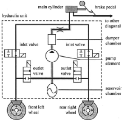
Diagnosing this subsystem requires solving a number of challenging problems:

• Obviously, this is a system with complex dynamics.
• Observations are sparse: there is not a single sensor in the hydraulic circuit (the level sensor for the braking liquid is of no help). Information about pressures can only be obtained indirectly from the (de-)acceleration of the wheels. However:
• For off-board diagnosis, available observations are inherently qualitative in nature and not temporally specified. Typical observations would be "one wheel

tends to lock up" (indicating too high pressure in the respective brake cylinder) or "the brake pedal is too soft" (as a result of an unusually low pressure in the main cylinder). Even more precise values of speed and acceleration present on-board do not help too much, since:

• Measurement of strongly influential exogenous factors (e.g. the state of the road surface) is impossible. In response to these conditions, we adopted an approach described in [Malik-Struss 96] using models that are stated in terms of qualitative deviations of variables and parameters from some unspecified and potentially changing nominal value.

It turns out that the "measurements" characterized above, enable the models to infer deviations in the pressure in different parts of the circuit. This trivially suffices to establish measurability for fault detection, but not measura­ bility for fault identification and localization. The reason lies in the lack of information about the derivatives of pressures which cannot be provided by the observations and the state-constraints. Basically, this information would help to detect significant inconsistencies because resistive elements like valves relate (deviations of) flow to ( devia­ tions of) pressure, whereas pipes and other containers link (deviations of) flow and (deviations of) derivatives of pressure.

The solution was indeed provided by exploiting CID­ constraints. However, they were not used for simulation of correct or faulty behavior modes, but to complement the observations in the following manner:

For each phase in the cycle (determined by valve positions), strict continuity can be assumed. Furthermore, we assume that there were no deviations when the phase was entered (this limits the applicability of the solution). If a deviation of a variable v was zero initially and different from zero after a while, then the CID-constraints tell us that there must exist a time interval during which both the deviation of v occurred and the derivative of v has a deviation with the same sign. In other words, CID­ constraints were combined with OBS to deliver information about derivatives.

This turned out to be fairly successful: for a sample of component faults, such as clogged or punctured valves, defect pump, and air included, fault localization was successful: the respective faults were included in the set of single fault diagnoses, sometimes as only possible ones.

Other case studies that use related approaches and shed a light on its utility, are reported in the literature: [Dressler 96] empirically discovered the possibility of fault detection via state checking in a prototype for diagnosing ballast water tank systems in off-shore platforms (a fairly sensor-rich system). [Chantler et al. 96] reports results on equivalence of integration-based and differentiation-based algorithms for the special case of numerical models. [Williams-Nayak 96] pursues a transition-oriented, as opposed to simulation­ oriented, approach to diagnosis and reconfiguration applied to the propulsion system of a space craft. [Malik-Struss 96] covers fault detection and identification in a simplified system (a controlled electric motor) with limited observability, but measurable derivatives based only on state checking.

6 Summary

As [Malik-Struss 96] states, "Diagnosis of dynamic systems does not necessarily require simulation". This paper presented theoretical foundations and practical considerations supporting model-based diagnostic systems that are confmed to using state constraints for consistency checking and do without temporal behavior constraints, or use them for purposes other than simulation. There are empirical results that provide evidence of the utility of such approaches, but also attempt steps towards identifying their limitations, particularly limitations that result from limited observability of the system. We hope that our analysis

• discourages overly "straightforward" approaches to model-based diagnosis,
• encourages more steps towards a systematic and thorough investigation leading to the design of diagnosis systems that are both well-founded and efficient,
• shows that such steps require a specific and detailed analysis of properties of models and predictive engines on the one hand and their interrelationship with observability on the other hand.

The benefit of these efforts will be beyond theoretical insight and result in widening the scope of feasible industrial applications which often involve dynamic systems.