Diagnosing Tree Structured Systems

1 Introduction

Since the beginning of model-based diagnosis research, several attempts have been made to make model-based diagnosis of large systems feasible. This has been done by introducing probability measurements ([dK91]), by computing a component focus as in [FF92; PG93], or by using special control strategies (e.g., [SD89; GRST89)). However, fault probabilities are not available in all do­ mains, and complete discrimination between diagnoses is also not possible in all examples.

Therefore in the past years, much effort has been spent on the development of faster diagnosis algorithms. In [FD95], an algorithm based on constraint satisfac­ tion for tree structured diagnosis systems was introduced whose performance, as the accompanying experimental evaluation showed, compared favorably with the algo­ rithms of Reiter [Rei87; GSW89] and de Kleer [dKW87] . A new algorithm for the diagnosis of general diagnosis systems was also presented in [Dar95] (who also presents some results on an abductive variant). It was shown that the algorithm behaves best if the system is tree structu­ red, but without experimental results. Other diagnosis algorithms such as [AFK88] are limited to single fault diagnosis and/or to a specific data structure such as boo­ lean algebra.

This paper presents a simple diagnosis algorithm desi­ gned for use on tree-structured systems. The algorithm description is given using standard model-based termi­ nology and we show results based on testing them with automatically generated examples. The experiment sho­ wed that the improvement compared to Reiters diagno­ sis algorithm depends on the ratio between number of components and number of inputs. Since there exists an inverse relation between the number of inputs and the number of diagnoses, the performance depends also on the number of computed diagnoses. Systems with many inputs can be diagnosed faster than systems with only one input.

The paper is organized as follows. In section 2, we give the basic definitions. We present the TREE_DIAG al­ gorithm in Section 3, discuss its complexity and show some experimental results in Section 4. Section 5 dis­ cusses the extension of TREE_DIAG to handle more general system topologies and fault modes. Finally, we summarize the results and discuss some open problems. Proofs have been omitted for brevity, see [SW96b] for details.

2 Basic Definitions

We define a diagnosis system as in [Rei87], except that we differentiate between components with inputs and those without inputs.

Definition 2.1 (System) A system is a tuple (SD,COMP U LEAF) where SD denotes the system description, COM P the set of components, and LEAF the set of components not connected to the outputs of another component.

LEAF components represent the input ports of the system and we assume they always behave correctly.

A function describing the behavior in terms of input and output ports is associated with every component. We start out by assuming that every component has only one output port. The function associated with the component can be accessed using June : COM P t-t FU NC. The arity of a function is given by arity :

FUNC r-+ IN. (For brevity we will write arity(C) in­ stead of arity(func(C)) .) Input ports of C are writ­ ten as ini(C) and the output port as out(C). Ports are assumed to have values, expressed by the function val: PORTS r-+ VALUES. Because there exists only one output for every component, we use val(C) instead of val( out( C)) for brevity. The system description uses the defined functions to express a diagnosis system. The behavior of components can be expressed by the rule

Connections between ports of components are also ele­ ment of the system description:

Every connection allows a value propagation:

The set of all components connected to input ports is denoted by in(C) = {C'Iout(C') = ini(C) E SD}. Note that for all leaf components L, in(L) = 0.

A diagnosis problem related to a given system can be stated by including a set of observations.

Definition 2.2 (Diagnosis Problem) Let

(SD, COM P U LEAF) be a system and OBS be obser­ vations. The tuple (SD,COMPULEAF,OBS) is said to be a diagnosis problem. We assume that all elements of LEAF have an associated observation.

The observations are given in terms of a function re­ turning the observed value of the component:

observed: COM P u LEAF r-+ VALUES.

A system is correct if the observed value is equal to the derived value for every component. We therefore introduce the rule

Diagnoses are defined in the usual manner.

Definition 2.3 (Diagnosis) 6. a subset of COM P is a diagnosis for (SD,COMP u LEAF,OBS) iff SD u OBS u {ok(C)I E COMP \ 6.} u {·ok(C)IC E 6.} is consistent.

Because leaf components only store input values for the system, they are not considered in 6.. The set of top components tops(SD,COMPULEAF) includes all components that are not used as input of other com­ ponents.

Definition 2.4 (Path) Let C1 , Cn be two components. A path connecting C1 with Cn is a sequence of com­ ponents [C1, ... , Cn] where each Ci+l is connected to an input of ci.

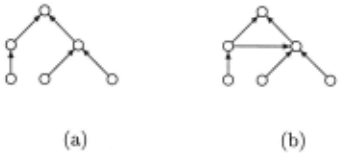
We can consider the diagnosis system as a directed graph whose vertices are components and whose edges are connections from an output of a component to the input of another component. We call the diagnosis sy­ stem acyclic if this graph contains no directed cycles. The set of all paths from one component to another is defined by paths(C1, C2) = {PIP = path(C1 , C2)}. We say a component C' is connected to C if there is a path from C' to C in the graph.

Tree structured systems have only one top component and from every other component to the top component there exists only one path. Figure 1 (a) shows a tree structured system, and (b) an acyclic one.

Definition 2.5 (Tree Structured Systems) A system ( S D, C 0 M P U LEAF) is tree structured iff tops(SD,COMPULEAF) = {C}/\ VC' E COMPULEAF: lpaths(C',C)I = 1.

Corollary 2.1 Every tree structured system is acyclic.

3 TREE...DIAG: An Algorithm for tree structured Systems

In this section we introduce the TREKDIAG dia­ gnosis algorithm for tree-structured systems. The ba­ sic idea is as follows. If the observed value of a com­ ponent is not equal to the output of the component (as computed using the assumption that all components work correctly), there must be an incorrect component in the system. First, the component itself can behave incorrectly, i.e., it is a single fault. Secondly the com­ ponent can be correct, but another component connec­ ted to the input can behave incorrectly. If this is the case, the inputs must have values leading to the obser­ ved output value. Therefore we introduce a function IN PUTS which computes all input values producing the observed value and call the diagnosis function re­ cursively on the input components using those values: INPUTS,(val) = {i E Def(f)lf(i) = val}i. All dia­ gnoses must be combined to give the overall diagnosis.

It is obvious that we do not need to compute all input tuples leading to the wrong output since we are only interested in minimal diagnoses. We must only use the tuples which are as close as possible to the original input tuple. For example, if we have an and gate with the input tuple (1, 1) and the observed output 0, we use the tuples (1 , 0) and (0, 1) for computing diagnoses.

1 Note that in many cases it is possible (and necessary) to impose further restrictions on the definition, depending on the properties and domain of f.

Before introducing the algorithm in detail, we de­ fine some auxiliary operators. For two diagnosis sets s, sl, Sz, the operator X is defined as:

1. Sx{}={}xS={} 2. sl X Sz = U·tESt {xl Uxz} · 2ES2

This definition can be extended to the general case, where n sets should be combined.

We also want to restrict diagnosis sets to contain only diagnoses up to a given size. For a diagnosis set S and ds EN, we write Slds ={DID E S 1\ IDI ~ ds}

In addition, we assume a function checked answe­ ring whether a component has been used for diagno­ sis or not . Before executing TREE..DIAG, checked answers false for all components. The TREE..DIAG algorithm uses a global variable, diags , to collect dia­ gnoses as they are constructed. The variable diags is initialized to { {} }. For a given diagnosis problem (SD ,COMP, LEAF,OBS), the algorithm is called by TREE...DIAG(top(SD, COM P)) .

Algorithm TREE..DIAG(C)

Evaluates every component, i.e., computes their out­ put values and calls the diagnosis algorithm if the com­ puted value is not equal to an observed value. It is assu­ med that observations exist for all leaf components. C .. . current Component, initially the top component Global constants: SD, COMP, LEAF, OBS Global variables: diagSize (prespecified max. diagnosis size) and diags {Diagnosis set, initialized to { {}})

IF C E LEAF THEN val (C) t- observed( C)); checked( C) t- true ELSE FORiE {1, ... , arity(C)} DO Vi t- TREE...DIAG(ini (C)) END FOR; V t- func(C)(VI, ... , Varity(C)); IF exists(observed(C)) AND V =f observed( C) THEN diags t- (diagsx DIAG(C,observed(C))) ldiagSize; val (C) t- observed( C) ELSE val(C) t-V END IF END IF

Algorithm DIAG(C,E)

Compute diagnosis by explaining differences between the computed and the observed behavior.

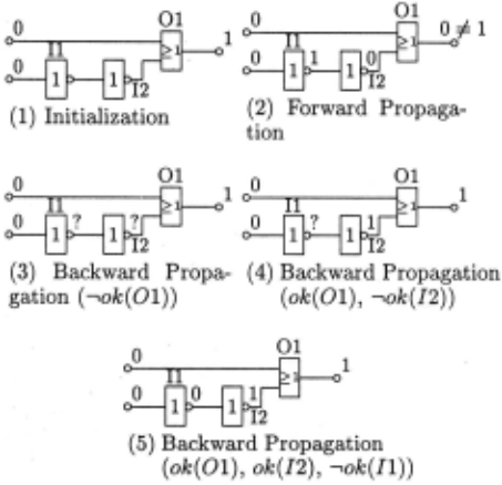
C . .. current Component E .. . Observed value Global constants: SD, COMP, LEAF, OBS Global variables: diagSize {Diagnosis size) and diags {Diagnosis set) IF checked( C) THEN IF val(C) = E THEN RETURN{{}} ELSE RETURN{} END IF ELSE checked( C) t- true IF E = val(C) THEN RETURN{{}} ELSE new_diags t- {{C}}; FOR (v1, .. . , Varity(C)) EINPUTS(SD,C,E) DO collected..diags t- { {} }; FORi t- 1 TO arity(C) DO collected..diags t- ( collected..diags x DIAG(ini(C),vi)) ldiagSize END FOR; new_diags t- new_diags U collected..diags END FOR; RETURN new_diags END IF END IF

We explain the operation of TREE..DIAG using a small example. Inverters are denoted by I x and or ga­ tes by Ox. Figure 2(1) shows the initialization of the system with observed values. The input observations are propagated to the output causing a discrepancy (see Figure 2(2)) . In Figure 2(3) the misbehavior is explained by assuming that 01 behaves incorrectly. In Figure 2(4), 01 is assumed to behave correctly, leading to the input vector (0,1) which can be explained by assuming that I2 is faulty. In Figure 2(5) backward propagation is done by assuming that I2 behaves correctly, causing Il to be incorrect.

The algorithm is sound and complete with regard to the definition of diagnosis.

Theorem 3.1 (Termination of TREE..DIAG) The TREE..DIAG algorithm halts on every tree structured diagnosis system.

Theorem 3.2 (Soundness and Completeness) The TREE..DIAG algorithm is sound wrt. the dia­ gnosis definition, i.e., every element D. E diags after the algorithm has terminated is a diagnosis. Also, the algorithm computes all minimal diagnoses.

We conclude the section with a brief discussion of the time complexity of the TREE..DIAG algorithm.

Theorem 3.3 (Time Complexity of TREE..DIAG) The maximum time complexity of the TREE..DIAG al­ gorithm is of order o(COMP. 2lCOMPI) .

It is worth noting that this worst time complexity is very unlikely to occur, because we only consider minimal diagnoses, and a limit on the desired diagnosis size can be specified. Practical application of TREE_DIAG to the diagnosis of digital circuits has shown that the algo­ rithm is highly efficient and can be used even for large examples (see Section 4). In the individual case, the time complexity of TREE_DIAG depends on the com­ ponent functions, the structure of the system, and the diagnosis size.

Theorem 3.4 (Time Complexity, Single Fault) The maximum time complexity of the TREE_DIAG al­ gorithm is of order o(jCOM Pi) if only single faults are searched for.

4 TREE.DIAG Implementation Results

TREE_DIAG was implemented in ParcPlace Visual­ works/Smalltalk 2.5. The experiments were run on a SPARCStation 10-30 with 96 MB main memory. Ex­ amples were generated automatically using only and, or' and not gates. The number of components and number of inputs, i.e., leaf components, serve as input parame­ ters. All listed. figures are based on searching for single faults. There are no further restrictions on the inter­ nal structure of the circuit (i.e., no symmetry or con­ stant depth of leaves). To allow a direct comparison of TREE_DIAG with other existing MBD algorithms, Reiter's HS-DAG and the SAB algorithm from [FD95] were also implemented.

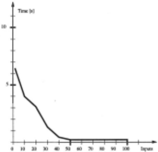
Figure 3 shows the amount of diagnosis time as a func­ tion of the number of components for circuits with the number of inputs set at half the number of internal com­ ponents. Results were derived by averaging over 100

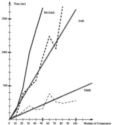
different example runs. Comparing the results leads to the conclusion that TREE_DIAG outperforms the two other MBD algorithms.

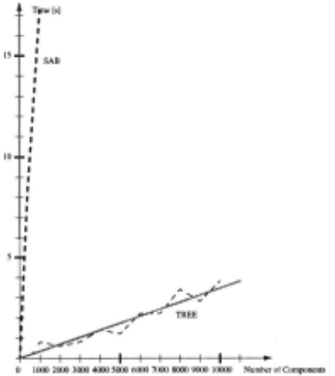
Figure 4 shows the performance of TREE_DIAG and SAB algorithm for systems with up to 10,000 diagnosis components. We can see that TREE_DIAG has a good response time even for very large systems. The maxi­ mum diagnosis time was always less than 13 seconds.

From the evaluation of TREE_DIAG, it is clear that the diagnosis time not only depends on the number of components, but also varies with the number of system inputs. Figure 5 shows the runtime behavior for the number of components fixed at 100 and examples gene­ rated for varying number of inputs. It can be seen that we obtain the best performance for TREE_DIAG if the number of inputs is equal to the number of components. In the worst case (1 input) the diagnosis system degene­ rates to a row of inverters where diagnosis discrimination is not possible without using additional measurements. Note that the time scale for this figure (and Figure 4) is significantly larger than for Figure 3. The time required for finding single faults is not zero, but merely stayed clearly below 1 second in all cases.

In the case where the number of inputs is small com­ pared with the number of components, the number of diagnoses returned is large, therefore many diagnoses are added to the diagnosis set of TREE_DIAG causing computational overhead. However, in summary our ex­ periments indicate that TREE_DIAG always performs better than the HS-DAG and SAB algorithm.

5 Extending TREE.DIAG

The TREE_DIAG algorithm can be extended in a num­ ber of ways. First, we can release the restriction that a system may only possess one output. Second, by ex­ tending the algorithm from trees to directed acyclic sy­ stems, including systems that contain components with multiple outputs. Finally, by combining directed acyclic systems with system descriptions using fault modes.

The assumption that a system possesses only one out­ put can be easily avoided, because every system with n outputs can be transformed to a system with one output by adding a component 6 with one output and n inputs with the following behavior:

out(6) = [val(in1(6)) , ... , val(i nn(6))]

6 will under all circumstances be assumed to work correctly.

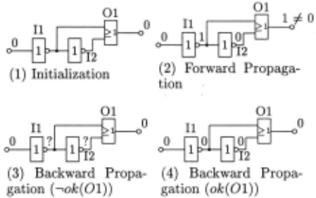
From now we will therefore assume that the diagnosis system has only one output. We will not present the DAG_DIAG algorithm in detail, but briefly discuss its basic characteristics. The structure of the algorithm is similar as for TREE_DIAG, except that in the gene­ ral case, back propagation alone will not be sufficient. Instead, in some cases additional forward propagation must be performed and included into the final results. Consider the example of Figure 6.

Phase (1) shows the initialization of the system with observed values. The input values are propagated to the output causing a discrepancy (see (2)). In phase (3), the misbehavior is explained by assuming that 01 behaves incorrectly, in ( 4) it is explained by the assumption that 01 behaves correctly, but that both inputs of 01 must be 0. In this case, we see that the value of 0 on the output I1 causes a discrepancy and that this happens also if 0 is propagated through !2. Therefore we can de­ rive one single fault {01} and one double fault {!1,!2}. Crucial to this example is that the value of 0 propagated back through 01 must afterwards be propagated forward through the cross connection via !2.

DAG_DIAG behaves similar to TREE_DIAG, ex­ cept in the case where the output of a component C is connected to more than one input. In this case, a new value is computed because the assumption that the component behaves correctly must be also propagated to the inputs of all components depending on C. If this propagation causes a discrepancy, the resulting diagno­ ses must be added to the diagnoses derived from back propagation.

The next extension is the handling of components with multiple outputs. Basically, a component C with two outputs out1 (C) and out2 (C) whose values are described by two functions such that val(out1(C)) = funcl(val(ii(,p(C)) and val(out2(C)) = func2(val(ii(,p(C))) respectively can be decomposed into two components C' and C", where val ( C') = funcl(val(ii(,p(C')) val(C") = junc2(val(ii(,p(C")), and inputs(C') = inputs(C") = inputs(C). A diagnosis D.' of the decomposed system is mapped into a diagnosis D. of the original system by stating that C E D. if C' E D.' or C" ED.'.

To introduce fault modes, the main alteration is to the IN PUTS function in DIAG, which receives a fault mode assumption for the current component as an additional argument and computes the possible input vectors for that particular fault mode.

Finally, note that the SAB algorithm was also app­ lied to cyclic systems by using a preprocessing stage ba­ sed on tree clustering [FD95], and the same process can be applied for the TREE...DIAG algorithm. However, in our particular application domain, software diagno­ sis [SW96a], the utility of this approach will often be limited, since significant structural alterations can be ex­ pected between diagnosis runs for different versions of a program, so that almost every diagnosis run will require a separate preprocessing stage. For cases where prepro­ cessing is not desired, the DAG ...DIAG algorithm is also superior to the Reiter algorithm (see [SW96b] for experi­ mental results). TREE...DIAG is sufficient, however, for the diagnosis of expressions in functional languages.

6 Conclusion

In this paper, we have presented a new diagnosis al­ gorithm. The TREE_j)IAG algorithm uses the tree structure of systems to subdivide the system and com­ bine the subdiagnoses afterwards. Experimental results using automatically generated examples have shown that the new algorithm improves on the HS-DAG diagnosis algorithm and the SAB algorithm [FD95], with perfor­ mance of the new algorithm (not too surprisingly) depen­ ding on the st.ructure of the diagnosed system. In our case, a conventional system description is used, in con­ junction with the requirement that a function IN PUTS must exist to compute inverses. There are no other re­ quirements on INPUTS (e.g., it could also be based on tables).

In addition, we have identified the number of system inputs as performance relevant factor: systems with many inputs can be diagnosed very quickly. Future work will include the implementation of the extended version of the algorithm that handles fault modes and the appli­ cation of the algorithm to software debugging [SW96a] .