
Diagnosing Tree-Decomposable Circuits
Proceedings of the Fourteenth International Joint Conference on Artificial Intelligence. Qualitative Reasoning and Diagnosis. Pages 1742-1748.
© 1995 International Joint Conferences on Artificial Intelligence
Abstract
This paper describes a diagnosis algorithm called structure-based abduction (SAB) which was developed in the framework of constraint networks [12]. The algorithm exploits the structure of the constraint network and is most efficient for near-tree problem domains. By analyzing the structure of the problem domain, the performance of such algorithms c~n be bounded in advance. We present empirical results comparing SAB with two modelbased algorithms, MBD1 and MBD2, for the task of finding one or all minimal-cardinality diagnoses . MBD1 uses the same computing strategy as algorithm GDE [9]. MBD2 adopts a breadth-first search strategy similar to the algorithm DIAGNOSE [24]. The main conclusion is that for nearly acyclic circuits, such as theN-bit adder, the performance of SAB being linear provides definite advantages as the size of the circuit increases.
- R. R . Bakker , M. Bourseau , and M. K. de Weger. Pragmatic reasoning in model-based diagnosis. In Working Notes of the Third International Workshop on Principles of Diagnosis, pages 107-116, Rosario, WA, USA, 1992.
- E. Charniak and S.E. Shimony. Probabilistic se- mantics for cost-based abduction. In Proceedings, AAAI-90, pages 106-111, Menlo Park, CA, 1990. AAAI Press/ The MIT Press.
- R. L. Childress and M. Valtorta. Polynomial-time model-based diagnosis with the critical set algo- rithm. In Working Notes of the Fourth International Workshop on Principles of Diagnosis, pages 166 - 177, University of Wales, Aberystwith , 1993.
- A. Darwiche. Conditional independence in ATMSs: Independence-based algorithms for computing la- bels and diagnoses. In Working Notes of the Fifth International Workshop on Principles of Diagnosis, pages 70-77, New Paltz, NY, USA, 1994.
- J. de Kleer. An assumption-based TMS. Artificial Intelligence, 28:127-162, 1986.
- J. de Kleer. Focusing on probable diagnoses. In Pro- ceedings of the Ninth National Conference on Arti- ficial Intelligence, pages 842-848, Menlo Park, CA, 1991. AAAI Press/ The MIT Press.
- J. de Kleer , A.K. Mackworth, and R. Reiter. Char- acterizing diagnoses and systems. Artificial Intelli- gence, 56:197-222, 1992.
- J. de Kleer and 0. Raiman. How to diagnose well with very little information. In Working Notes of the Fourth International Workshop on Principles of Diagnosis, pages 160-165, University of Wales, Aberystwith, 1993.
- J. de Kleer and B. C. Williams. Diagnosing multiple faults . Artificial Intelligence, 32:97-130, 1987.
- A. Dechter and R. Dechter. Structure-driven al- gorithms for truth maintenance. Artificial Intelli- gence , 1985.
- R. Dechter. Constraint networks. In Encyclopedia of Artificial Intelligence, pages 276-285.
- J. Wiley, New York, second edition, 1992.
- R. Dechter and A. Dechter. Belief maintenance in dynamic constraint networks. In Proceedings, AAAI-88, pages 37-42, Menlo Park, CA, 1988. AAAI Press/ The MIT Press.
- R. Dechter, A. Dechter, and J. Pearl. Optimization in constraint networks. In R.M. Olivier and J .Q. Smith, editors, Influence Diagrams, Belief Nets and Decision Analysis, pages 411-425. J. Wiley, New York, 1990.
- R. Dechter and J. Pearl. Tree clustering for con- straint networks. Artificial Intelligence, 38:353-366 , 1989.
- Y. El Fattah and R. Dechter. Empirical evalua- tion of diagnosis as optimization in constraint net- works. In Working Notes of the Third International Workshop on Principles of Diagnosis, pages 149- 158, Rosario, WA, USA, 1992.
- H. Freitag and G. Friedrich. Focusing on indepen- dent diagnosis problems. In Proceedings of the Third International Conference on Principles of Knowl- edge Representation and Reasoning (KR), pages 521-531 ' 1992.
- G. Friedrich, G. Gottlob , and W. Nejdl. Physical impossibility instead of fault models. In Proceed- ings, AAAI-90, pages 331-336, Menlo Park, CA , 1990. AAAI Press/ The MIT Press.
- H. Geffner and J. Pearl. An improved constraint propagation algorithm for diagnosis. In Proceedings, IJCAI-87, pages 1105-1111, 1987. IJCAI
- M. R. Genesereth. The use of design descriptions in automated diagnosis. Artificial Intelligence, 24:411- 436, 1984.
- D. Maier. The Theory of Relational Databases. Computer Science Press, Rockville, MD, 1983.
- I. Mozetic. A polynomial-time algorithm for model- based diagnosis. In B. Neumann, editor, Proceeding of the 1Oth European Conference on Artificial Intel- ligence (EGA! 92}, pages 729-733, New York, 1992.
- J. Pearl. Probabilistic Reasoning in Intelligent Sys- tems: Networks of Plausible Inference. Morgan Kaufman, San Mateo, CA, 1988.
- Y. Peng and J.A. Reggia. Abductive Inference Mod- els for Diagnostic Problem Solving. Springer-Verlag, Berlin, 1990.
- R. Reiter. A theory of diagnosis from first principles. Artificial Intelligence, 32:57-95, 1987.
- P. Resnick. Generalizing on multiple grounds: Per- formance learning in model-based troubleshooting. Technical Report AI-TR 1052, MIT Artificial Intel- ligence Laboratory, February 1989.
- E. Santos, Jr. On the generation of alternative ex- planations with implications for belief revision. In Proceedings, Uncertainty in Artificial Intelligence, pages 339-347, 1991.
References were extracted automatically from the PDF and may contain errors.
Full text extracted automatically from the PDF; figures, tables and equations may differ. The PDF is the version of record.
1 Introduction
Generally speaking, diagnosis is a form of abduction or inference to the best explanation. Explanations are those minimal sets of value instantiations that are consistent with the model and the observations, and best explana tions are those that optimize some desirability measure. Some common measures are minimal cardinality [19], parsimonious covering theory [23], most probable expla nation [22] and minimal cost proofs [2]. A well-defined relation be'tween cost-based abduction and belief revi sion in probabilistic networks has been shown [2], and also algorithms based on systems of linear constraints have been proposed [26] .
Diagnosis, when viewed as cost-based abduction, can be formulated as an optimization task in the framework of constraint networks [12; 11; 18]. The advantage of such formulation is that all algorithms and heuristics developed within that framework can be exploited. In
*This work was supported in part by the NSF (grant IRI9157636), the Air Force Office of Scientific Research (grant AFOSR 900136), Toshiba of America, Xerox, Northrop and Rockwell.
Rina Dechter
Computer Science Department University of California at Irvine Irvine, CA 92717 ( dechter@ics.uci.edu)
particular, it was shown that when a constraint network is acyclic, an optimal solution can be found in linear time [13]. Tailoring this algorithm to diagnosis results in an algorithm called structure-based abduction (SAB) [12], which will be empirically investigated here. The perfor mance of SAB is compared with two model-based diag nosis algorithms called here MBD1 and MBD2. MBDl uses the same strategy for finding predictions and con flicts as GDE [9]. MBD2 is a focused version of MBDl geared toward computing minimal-cardinality diagnoses. MBD2 adopts a breadth-first search strategy for search ing the hypotheses space and then computes conflicts sequentially, as in DIAGNOSE by Reiter [24].
The main contribution of this work is in illustrat ing how the task of diagnosis can be performed effi ciently for circuits whose structure corresponds to nearly acyclic networks. Note that model-based diagnosis algo rithms like GDE [9] can take an exponential time even on acyclic circuits (see Resnick [25]). We present results of experiments on a parameterized circuit that general izes Resnick's circuit showing instances where the GDE like algorithm (MBD1) explodes in time and space while SAB is able to compute diagnoses efficiently for all in stances. We then show how SAB can be applied to circuits whose structure is cyclic by using tree cluster ing [14] as a preprocessing phase. Applying tree. clu.s tering to cyclic circuits is known to be exponential m the cluster's sizes. We give empirical results on a pa rameterized cyclic circuit showing that even if relatively expensive, it is worthwhile doing tree clustering once so that all future diagnosis tasks are performed efficiently.
The structure of the paper is as follows. Section 2 reviews basic definitions and presents two model-based diagnosis algorithms: MBD1, MBD2. Section 3 formu lates diagnosis as optimization in constraint networks and describes algorithm SAB, and section 4 describes the tree clustering task. Section 5 presents empirical re sults, section 6 provides discussion and related work, and section 7 concludes.
2 Model-Based Diagnosis
Following [7] we define model-based diagnosis in terms of a triple (SD, COM PS, OBS) where SD, the system description, is a set of first-order sentences; COM PS, the system components, is a set of constants; OBS, the observations, is a set of first-order sentences. Intuitively, a diagnosis is a subset of components ~ C COM PS such that assuming that each component in ~ is faulty while the components in COM PS- ~ are not faulty, is consistent with the model and the observations. A diagnosis ~ for (SD, COM PS, OBS) is minimal if it does not contain a proper subset diagnosis.
Two diagnosis algorithms, MBD1 and MBD2, are ex amined, and will be described informally due to space restrictions. Algorithm MBD1 is a variant of GDE [9] . It works as a three-step process. In step 1, predic tions are computed by a form of constraint propagation, which although generally incomplete, is complete for re stricted languages such as trees and Horn theories. In step 2, all minimal conflict sets (nogoods) are enumer ated by identifying those "environments" leading to con flicts between predictions and observations. In step 3, all minimal-cardinality diagnoses are computed as the minimal-cardinality covers of all the conflict sets.
The worst-case time and space complexity for find ing all minimal conflict sets is clearly exponential in ICOM PSI . Since the task of finding a minimal cover to a set of subsets is known to be N ?-complete (even when each subset has at most two elements), the result ing worst-case complexity of the algorithm is likely to be (if P # N P) exponential.
The second diagnosis algorithm MBD2 reverses the steps of MBDl. It first generates a hypothetical diag nosis and then determines whether any conflicts remain unexplained by that hypothetical diagnosis. If such a conflict is found then the hypothesis is extended to cover each component in the new conflict. If such a conflict does not exist, the hypothesis is a minimal diagnosis. All other minimal-cardinality diagnoses are found by check ing each of the remaining hypotheses as to whether it can explain all the conflicts. MBD2 is a version of the algorithm DIAGNOSE by Reiter [24] modified for com puting the minimal cardinality diagnoses.
3 Diagnosis as Optimization
Given a set of variables Xt, .. .', Xn each having a finite set of domain values dom(X!), ... , dom(Xn) , a constraint network C N is a set of relations {It, ... , rm}, called con straints, each defined on a subset of variables St , ... , Sm. A relation over a subset of variables X;,, ... , X;i is a sub set of the cartesian products of their domains. A solution to C N is an assignment of a value to each variable sat isfying all the constraints. A constraint network can be associated with the set of all its solutions. Formally,
sol(CN) = {t = (Xt = Xt, ... , Xn = Xn)IVj, tsi E lj }, when ts stands for the projection of a tuple t on a subset of variables S. For certain applications, it is useful to define a cost function over all solutions. A simple cost function associates a cost c(X = x) with each value of a variable, and the cost of a solution is the sum cost over all (variable, value) pairs. The optimization task is to find a solution having an optimal cost (largest or smallest).
To capture the diagnosis task, we map the triple (SD, COM PS, OBS) into the relational framework as fol lows. The system description SD will be described in terms of two sets of variables: the system variables, Xt, ... , Xn, which are the inputs and outputs of all components with their associated finite domain values, dom(Xt), ... , dom(Xn) , and the assumption variables, A = {At, . .. , Am}, each associated with a component Cj E COM P S and describing its functioning status. In the simplest case, these are hi-valued vari ables in dicating whether the component is normal (value 0) or abnormal (value 1). In the more involved case, they can index different fault models. Each component ( Cj) input-output behavior under normal and abnormal con ditions are described by a constraint lj. Thus, the con straint 'i is defined over the set Rj = { Aj} U Sj , where Sj is the set of input and output variables for compo nent Cj. The observations OBS is described by forc ing value assignments for the corresponding variables. Non-zero costs are associated with assumption variables only. An abnormal component is assigned a cost of 1 [i .e., c(Aj = 1) = 1], while a normal component has a zero cost [i.e., c(Aj = 0) = 0] .
Given a model description and a set of observations, the diagnosis task is to construct an explanation , namely, an assumption tuple (At = at, ... , Am = am) that can be extended to a consistent solution (Xt = Xt, ... , Xn = Xn,At =at , . . . ,Am = am) · The cost of an explanation is the sum of the costs associated with the assumption variables. That is,
The task of finding a minimal-cardinality diagnosis cor responds to a minimum-cost solution since only faulty components are assigned a positive cost in the constraint network formulation .
The topology of a constraint network can be depicted by its dual graph. A dual graph represents each con straint by a node and associates a labeled arc with any two nodes that share variables. If the dual constraint graph is a tree (called a join tree) or can be transformed into a tree by removing redundant arcs (in linear time), then the constraint network is said to be acyclic [20] . In that case, a consistent solution or an optimal solution can be assembled in linear time.
Example 3.1 Consider the circuit in Fig. 1a, which has two AND-gates AND-1 , AND-2 connected to an OR-gate OR-1. We model this circuit using three bi-valued as sumption variables, At , A2 , A3, whose values, zero or one, indicate whether the respective gate AND-1 , AND-2 , and OR-1 , is normal or abnormal. Fig. 1b shows the dual graph for the circuit , where a node corresponds to the
| A1 | Vl | V2 | V3 | Cost |
|---|---|---|---|---|
| 0 | 0 | 0 | 0 | 0 |
| 0 | 0 | 1 | 0 | 0 |
| 0 | 1 | 0 | 0 | 0 |
| 0 | 1 | 1 | 1 | 0 |
| 1 | X | X | X | 1 |
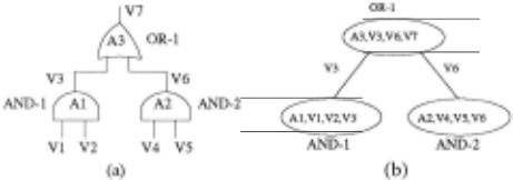
Table 2: SAB

set of input-output variables including its associated as sumption variable. The explicit constraint for each node is given as a table of allowed tuples.
Constraint AND-1 is given in Table 1, where the values marked with an X correspond to "don't care" conditions (either 0 or 1). Given the set of observations {V1 = 0, V2 = 1, V4 = 1, V5 = 1, V7 = 0}, there are two best explanations, both having cost 1. { A1 = 0, A2 = 1, A3 = 0} corresponding to a single-fault of AND-2, and {A 1 = 0, A2 = 0, A3 = 1} corresponding to a single fault of OR-1. Notice that multiple-fault explanations also exist, but they have higher costs.
Table 2 presents algorithm SAB for a join-tree net work. In the bottom-up step, pointers are created from each tuple t of a parent node to each of a set of mini mizing tuples for each child node. The complexity of the bottom-up phase of the algorithm is O(n · t ·logt), where n is the number of components (nodes of the join tree) and t is the number of tuples. Details about the algo rithm and arguments for correctness are given in [12; 13; 10].
4 Tree Clustering
For completeness we present in Table 3 the main steps in the tree-clustering algorithm [14]. Tree clustering is based on a triangulation algorithm which transforms any graph into a chordal graph by adding edges. The maxi mum cliques of the resulting chordal graph are the clus ters necessary for forming an acyclic CN. The relation
Table 3: Tree ClusteriJ!g_
Input: A cyclic constraint network T.
Output: A join tree representation ofT.
- Order the nodes (in a maximum cardinality order ing (mco) and use a triangulation algorithm to gener ate a chordal graph for T.
- Identify the maximum cliques C1 , ... , Ct and in dex them by the order of their earliest variable in the ordering.
- Return the join tree resulting from connecting each C; to a Cj whose index j > i and with whom it shares the largest set of variables.
- Compute for each node in the tree the set of tu ples satisfying all constraints on the clique and arc consistency with the children.
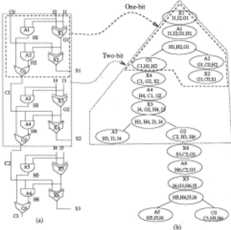
for each cluster (step 3) is computed by assigning the input constraints to the various clusters of the join tree and finding for each clique all tuples satisfying those con straints. The complexity of this step dominates the al gorithm's performance and is exponential in the clique's SIZe.
Example 4.1 Figure 2 shows the join tree for the three bit adder. We note the recursive nature of the tree, and the fact that the maximum clique size is independent of the number of bits of the adder.
5 Empirical Evaluation
5.1 Acyclic Circuits 1
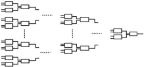
The first set of experiments is restricted to a family of circuits whose CN is acyclic. We compare the perfor mance of SAB to MBD1 on the task of computing all minimal-cardinality diagnoses on the parameterized cir cuit b(p, k), shown in Figure 3. The circuit has n = 2k-1 components and k layers numbered 1, 2, .. , k from the leaves to the root. The component types are indepen dent random variables and are either AND or OR gates. A component in an odd (even) layer is an AND (ORJ with probability p, OR (AND) with probability 1 - p. The circuit b(p, k) is acyclic and can have a worst-case exponential number of minimal conflicts. 3
1 Preliminary experimental results appear in [15]
Method
For every circuit, we generate the inputs as independent random variables each having the value 1 with proba bility q and 0 with probability 1- q. Then the correct output is determined and reversed. The observation con sists of the inputs and the faulty output . We feed the same set of problems to both SAB and MBD1 and record their respective performances. We limit the space and time that can be used by M BD1 to make the experi ments feasible. When the limits are reached, MBD1 is terminated with no solution . Each experiment consists of M(= 2) circuits each with N(= 5) input-output sce narios. The performance is averaged over the N · M problem instances. The circuits considered have com ponents ranging from 3 to 511. Our experiments were conducted using Quintus Prolog on Sun 670MP.
2 A special case of the circuit , b(l, k) , was developed by [25].
3 Although the number of conflicts can be exponential for certain inputs, this does not imply that it is the case for most inputs.
Results
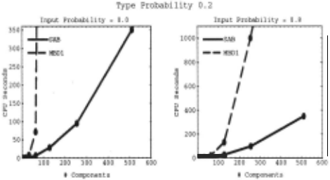
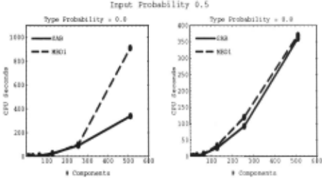
The results of the experiments, given in Figures 4 and 5, display the average CPU times used by SAB and MBD 1 for computing all minimal-cardinality diagnoses. In Fig ure 4, the input probability is varied while the type prob ability (the type of the component being an AND or an OR gate) is fixed at 0.2. In Figure 5 the type probabil ity is varied while the input probability is fixed at 0.5. Those figures show that MBD1 becomes inefficient for computing the diagnoses for moderately sized circuits . Points that are not shown for MBD1 correspond to cir cuit sizes for which MBD1 failed on all problem instances because its space (or time) requirement exceeded avail able resources. For such problems , the space required by MBD1 's caching during the prediction phase had ex hausted the available resource limit, set at 10,000 pre dictions. The points shown for MBD1 give the average CPU seconds over the solved-problem instances.
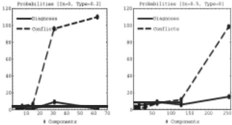
As observed from Figures 4 and 5, MBD1 is sensi tive to the type of the randomly generated circuits and to the probability of the inputs . For circuits having 63 components and type probability 0.2, changing the in put probability from 0 to 0.8 resulted in a change in the average CPU seconds from 71.5 to 19.5 for MBD1 and 6.95 to 8.04 for SAB. The coefficient of variation (the ratio of the standard deviation to the mean) of the CPU seconds is also an order of magnitude higher for MBD1 than for SAB (around 50% for MBD1 and 5% for SAB.) It is also observed that for small sized circuits , MBD1 's performance is comparable to SAB's. Figure 4 shows that for input probability close to 0 or 1, MBD1 is gen erally slower than SAB. On the other hand, for input probability 0.5, MBD1 is very close to SAB for some circuits (Figure 5) . As suggested by theoretical analy sis, it appears that MBD1's performance is correlated with the number of conflicts, while SAB's performance is affected by the number of diagnoses . On average, the performance of MBD1 relative to SAB degrades as the number of conflicts relative to the number of diagnoses increases. Fig. 6 shows the average number of conflicts and diagnoses for two cases: one where SAB is consis tently faster (type probability 0.2 and input probabil ity 0), and the other where MBD1 is sometimes faster (type probability 0 and input probability 0.5) . The fig ure clearly shows that MBD1 is at a disadvantage with respect to SAB when there is a large number of conflict sets but a small number of minimal-cardinality covers. On the other hand, MBD1 is at some advantage with respect to SAB when the number of conflicts is small while the number of diagnoses is relatively large.
5.2 Cyclic Circuits
To overcome the space problem of the ATMS caching used in MBD1 in the rest of our experiments we used algorithm MBD2 since it avoids MBD1's memory prob lem. The algorithm is still time exponential.
In this section we demonstrate that even if the struc ture of the problem is not acyclic, diagnosis and abduc tion may still be accomplished efficiently by transforming the problem into a tree using tree clustering and subse quently solving by SAB. In this set of experiments the N-bit adder circuit, whose structure is cyclic, is consid ered. An N-bit adder has 5 N components and can be modeled by a network having 12 N + 1 variables.
Tree Clustering
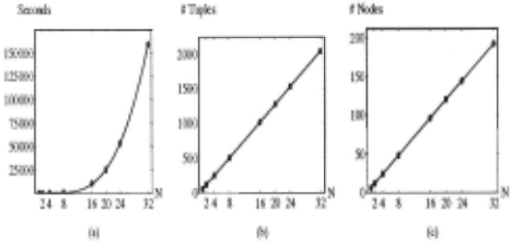
Tree clustering is performed on the circuit prior to diag nosis. Figure 7a gives the time of tree clustering which increases polynomially with N. We also see that the to tal number of tuples increases linearly with N (Figure 7b), and the number of nodes of the join tree (number of cliques) grows linearly with N (Figure 7 c).
Method
As in the acyclic case, we generate the inputs as inde pendent random variables each having the value 1 with probability q and 0 with probability 1- q. The outputs are computed by propagating the inputs through the component's constraints. Two types of experiments are conducted. In one, a single output is randomly selected and inverted. In the second set of experiments, multi ple outputs are randomly selected (half of the outputs, on average) and inverted. In all experiments, the ob servation consists of all input, all the correct and faulty outputs. The observation consists of all input, all cor rect outputs and the single faulty output. We record the performance of both SAB and MBD2 on each problem instance generated that way. An experiment consists of a set of 20 problem instances for each circuit and their performances is averaged over the problem set. A time limit of 1000 seconds per problem is set for MBD2.
Results
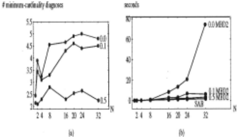
Figure 8 shows the performance of SAB and MBD2 for single faulty output when varying the input proba bilities. A single faulty output corresponds to the case where components fail with a very small probability. The minimal-cardinality diagnoses consist of only single fault diagnoses. Figure 8a shows the average number of min imal cardinality diagnoses versus the circuit size N for three input probabilities. The average number of diag noses is small ( < 5) and decreases towards equal proba bilitys for '0' and '1' (0.5). Figure 8b shows the average time for computing all minimal-cardinality diagnoses by SAB and MBD2. The figure shows that SAB is highly ef fective resulting in a large speed-up as N increases. The speed-up is particularly significant for the case where all inputs are zero. For input probability 0.5, the average .
time is nearly identical for both SAB and MBD2. For a 16-bit adder (80 components) and inputs zeros, SAB's performance time ranges between 0.72 and 0.80 seconds, while on the same set of problems algorithm MBD2 takes between 2.3 and 11.7 seconds. For a 32-bit adder (160 components) and when all inputs are zeros, the time by SAB ranges between 1.62 and 3 sec., while by MBD2 between 30.4 and 155 sec.
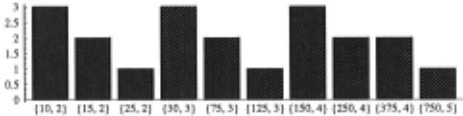
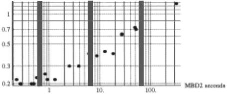
For multiple faulty output, the number of minimal diagnoses increases exponentially with N and their car dinality is greater than 1. Problem instances on an 8bit adder had 3750 minimal-cardinality diagnoses for in put probability 0 and 18750 for input probability 0.1. This corresponds to the case where components fail with non-small probability. MBD2 was able to compute di agnosis up to a four-bit adder but exceeded the limit on the eight-bit adder, even when computing one diag nosis. SAB, on the other hand, computed all diagnoses for the eight-bit adder , and it took only 59.82 seconds to compute all 18750 diagnoses in one particular prob lem instance. For the four-bit adder, where comparison can be made between SAB and MBD2, we plotted the histogram of the distribution of 20 problem instances as a function of the number of diagnoses and their cardi nality (Figure 9) . We also give a scatter diagram for the time to compute all diagnoses by SAB and MBD2 on each problem instance (Figure 10). Figure 9 shows that the cardinality of the diagnoses ranged between two and five and that number of minimal-cardinality diag noses ranged between 10 and 750. Figure 10 shows that SAB was an order of magnitude more time efficient than MBD2 . MBD2's time ranged between 0.23 seconds and 325.85 seconds while SAB's time ranged between 0.2 sec onds and 1.27 seconds. MBD2 required 325.85 seconds to solve a hard problem having 750 diagnoses of cardi nality 5 (Figure 9) and took only 0.23 seconds to solve an easy problem having 10 diagnoses of cardinality 2 (Fig ure 9). SAB required 1.27 seconds for the hard problem instance, while 0.22 seconds for the easy one.
6 Discussion and related work
The common approach to model-based diagnosis has widely been based on the language of propositional logic [7] and the reasoning machinery of the ATMS [5]. The main advantage of using constraint network tech niques for diagnosis is that it allows the structure of the system to be effectively exploited and the complexity of computation to be bounded in advance. For example, the circuit in Figure 3 may have an exponential num ber of minimal conflict sets (exponential in the square root of the number of circuit components [25]), yielding an exponential time for computing diagnoses by MBDl. Our algorithm, on the other hand, is linear time for that circuit and its efficiency can be determined by a sim ple analysis of the circuit structure, prior to execution . MBD2 will still perform poorly on this problem instance due to the time needed for checking that a current hy pothetical diagnosis covers all conflicts. For near-tree networks , the computation done vy tree-clustering can be viewed as replacing the computation of all conflict sets in MBD1 and MBD2. However, while the number of conflicts, on which MBD1 and MBD2's performance depend, is hard to predict in advance, the cost of tree clustering can be predicted by analyzing the structure of the circuit.
Several methods have been proposed [8; 1] to avoid the combinatorial explosion of the early GDE-style compu tation [9] . In those works, various heuristics are adopted that trade off completeness with efficiency. Algorithms have been proposed to compute the first k minimal (not necessarily minimal-cardinality) diagnoses (for fixed k) in polynomial time [17; 21; 3]. In [16] an approach called "structural focusing" is presented based on identifying those parts of the system whose diagnoses are indepen dent of the remaining parts of the system. An "inde pendent diagnosis problem" in [16] depends not only on the structure of the circuit but also on the observation instance of the diagnosis problem. A typical example is an N-bit adder problem where all inputs and outputs are set to 0 except for the output carry of the last one-bit adder. That circuit with that observation instance has first been suggested in [6] to motivate work on focusing on probable diagnosis. Unlike those focusing approaches, our approach only depends on the structure of the cir cuit . A structural notion of independence similar to ours has also been advocated recently and several versions of a diagnosis algorithm are given in [4].
7 Summary and conclusions
SAB is a diagnosis algorithm that exploits the structure of the problem when computing minimal-cardinality di agnoses. For problems containing no cycles, SAB is time and space linear. MBD1 (similar to GDE [9]) can find all minimal diagnoses and is not restricted by the struc ture of the problem. MBD2 is an incremental version of MBD1 that focuses on minimal cardinality diagnoses . Since SAB's complexity is time and space linear while MBD1's (MBD2's) is exponential, we expected a signif icant performance gain by SAB over MBD1 (MBD2). Two sets of experiments are conducted. The first set compares the diagnostic performance of SAB and MBD 1 on a class of randomly generated acyclic circuits. The second set compares SAB and MBD2 for diagnosing cir cuits containing cycles (N-bit adder) with randomly gen erated inputs and multiple faults. The first experiments show that algorithm SAB is superior to MBD1 for most problem instances. Depending on the circuit type and the input probabilities, there exists a critical circuit size
(in the order of 100 components) beyond which MBD1 becomes inefficient in space and time and thus diagnoses cannot be computed (for at least one generated prob lem). Unlike MBD1, SAB was able to compute the di agnoses for all circuit sizes studied (3 to 511 components) and all problem instances. In comparison to SAB, MBD1 was markedly sensitive to variations in the probabilities of the inputs and the types of circuits studied. In gen eral, MBD1 seems to be at a disadvantage with respect to SAB when the number of conflict sets is large and the number of minimal-cardinality covers is small. On the other hand, MBD1 is at some advantage when the num ber of conflicts is small while the number of diagnoses is relatively large. The second set of experiments show that even when relatively expensive, it is worthwhile do ing tree clustering once so that all future diagnosis tasks are performed efficiently. The main conclusion is that for nearly acyclic circuits, such as the N-bit adder, the performance of SAB, being linear, provides a definite ad vantage as the size of a circuit increases and the number of minimal conflicts or diagnoses becomes too large.
@inproceedings{ijcai1995p224,
  title     = {Diagnosing Tree-Decomposable Circuits},
  author    = {Fattah, Yousri El and Dechter, Rina},
  booktitle = {Proceedings of the Fourteenth International Joint Conference on
               Artificial Intelligence, {IJCAI-95}},
  publisher = {International Joint Conferences on Artificial Intelligence},
  editor    = {Chris S. Mellish},
  pages     = {1742--1748},
  year      = {1995},
  note      = {Qualitative Reasoning and Diagnosis},
  url       = {https://ijcai.org/proceedings/1995/224},
}
TY - CPAPER TI - Diagnosing Tree-Decomposable Circuits AU - Fattah, Yousri El AU - Dechter, Rina T2 - Proceedings of the Fourteenth International Joint Conference on Artificial Intelligence, IJCAI-95 PB - International Joint Conferences on Artificial Intelligence PY - 1995 SP - 1742 EP - 1748 UR - https://ijcai.org/proceedings/1995/224 ER -Copied
Machine-readable versions of this paper, for tools and AI agents:





