
Responsibility and Blame: A Structural-Model Approach
Proceedings of the Eighteenth International Joint Conference on Artificial Intelligence. Pages 147-152.
© 2003 International Joint Conferences on Artificial Intelligence
Abstract
Causality is typically treated an aU-or-nothing concept; either A is a cause of B or it is not. We extend the definition of causality introduced by Halpern and Pearl 2001a to take into account the degree of responsibility of A for B. For example, if someone wins an election 11-0, then each person who votes for him is less responsible for the victory than if he had won 6-5. We then define a notion of degree of blame, which takes into account an agent's epistemic state. Roughly speaking, the degree of blame of A for B is the expected degree of responsibility of A forB , taken over the epistemic state of an agent.
- [Chockler eta!. , 2003] H. Chockler, 1. Y. Halpern, and 0. Kupferman. Causality and responsibility in temporal logic model checking, Unpublished manuscript Available at http://www.cs.corne!Ledu!home/halpern/papers/resp.ps, 2003. Link
- [Collins eta!., 2003] J. Collins, N. Hall, and L.A. Paul, ed- itors. Causation and Counterfactuals, MIT Press, Cam- bridge, Mass., 2003 .
- [Eiter and Lukasiewicz, 2002a] T Eiter and T. Lukasiewicz. Causes and explanations in the structural-model approach: tractable cases. In Proc. Eighteenth Conference on Un- certainty in Artificial Intelligence (UAI 2002) , pages 146- 153, 2002.
- [Eiter and Lukasiewicz, 2002b] T. Eiter and T. Lukasiewicz. Complexity results for structure-based causality. Artificial Intelligence, 142(1):53-89, 2002. IJCAI
- [Hall, 2003] N . HalL Two concepts of causation. In
- Collins, N. Hall, and L.A. Paul, editors, Causation and Counterfactuals. MIT Press, Cambridge, Mass., 2003 . Halpern and Pearl, 2001 a]
- Y. Halpern and 1. PearL Causes and explanations: A structural-model approach. Part I: Causes. In Proc. Seventeenth Conference on Un- certainty in Artificial Intelligence (UAI2001), pages 194- 202, 2001, The full version of the paper is available at http://www.cs.corne!Ledu/home/halpern. Link
- [Halpern and Pearl, 2001b] J. Y. Halpern and J. PearL Causes and explanations: A structural-model approach. Part II: Explanations. In Proc. Seventeenth International Joint Conference on Artificial Intelligence (IJCAI '01) , pages 27-34, 2001. The full version of the paper is avail- able at http://www.cs.corne!Ledu!home!halpern. IJCAI Link
- [Hume, 1739] D. Hume. A Treatise of Human Nature. John Noon, London, 1739.
- CAUSALITY
- [Papadimitriou, 1984] C.H. Papadimitriou. The complexity ofunique solutions. Journal of ACM, 31:492-500, 1984.
- [Pearl, 2000] J. PearL Causality: Models, Reasoning, and Inference . Cambridge University Press, New York, 2000.
- [Stockmeyer, 1977] L. J. Stockmeyer. The polynomial-time hierarchy. Theoretical Computer Science, 3: 1-22, 1977.
- [Zimmerman, 1988] M. Zimmerman. An Essay on Moral Responsibility. Rowman and Littlefield, Totowa, NJ., 1988.
References were extracted automatically from the PDF and may contain errors.
Full text extracted automatically from the PDF; figures, tables and equations may differ. The PDF is the version of record.
1 Introduction
There have been many attempts to define causality going back to Hume 1739, and continuing to the present (see, for exam ple, [Collins eta!. , 2003; Pearl, 2000] for some recent work). While many definitions of causality have been proposed, all of them treat causality is treated as an aU-or-nothing concept. That is A is either a cause of B or it is not. As a consequence, thinkidg only in terms of causality does not at times allow us to make distinctions that we may want to make. For example, suppose that Mr. B wins an election against Mr. G by a vote of 11- 0. Each of the people who voted for Mr. B is a cause of him winning. However, it seems that their degree of resp~n sibility should not be as great as in the case when Mr. B wms 6-5.
In this paper, we present a definition of responsibility that takes this distinction into account. The definition is an ex tension of a definition of causality introduced by Halpern and Pearl 200la. Like many other definitions of causality going back to Hume 1739, this definition is based on counterfactual dependence. Roughly speaking, A is a cause . ~f B ~f, had A not happened (this is the counterfactual cond1t1on, smce -:4 did in fact happen) then B would not have happened. As 1s well known this naive definition does not capture all the sub tleties invol~ed with causality. In the case of the 6- 5 vote, it Joseph Y. Halpern*
*Supported in part by NSF under grant CTC-0208535 and by the DoD Multidisciplinary University Research Initiative (MURI) program administered by ONR under grant NOOO 14-01-1-0795.
Department of Computer Science Cornell University
Ithaca, NY 14853, U.S.A.
Email: halpem@cs.comell.edu
is clear that, according to this definition, each of the voters for Mr. B is a cause of him winning, since if they had voted against Mr. B, he would have lost. On the other hand, in the case of the 11-0 vote, there are no causes according to the naive counterfactual definition. A change of one vote does not makes no difference. Indeed, in this case, we do say in natural language that the cause is somewhat "diffuse".
While in this case the standard counterfactual definition may not seem quite so problematic, the following example (taken from [Hall, 2003]) shows that things can be even more subtle. Suppose that Suzy and Billy both pick up rocks and throw them at a bottle. Suzy's rock gets there first, shattering the bottle. Since both throws are perfectly accurate, Billy's would have shattered the bottle had Suzy not thrown. Thus, according to the naive counterfactual definition, Suzy's throw is not a cause of the bottle shattering. This certainly seems counter to intuition.
Both problems are dealt with the same way in [Halpern and Pearl, 2001a]. Roughly speaking, the idea is that A is a cause of B if B counterfactually depends on C under some con tingency. For example, voter 1 is a cause of Mr. B winning even if the vote is 11-0 because, under the contingency that 5 of the other voters had voted for Mr. G instead, voter 1 's vote would have become critical; if he had then changed his vote, Mr. B would not have won. Similarly, Suzy's throw is the cause of the bottle shattering because the bottle shattering counterfactually depends on Suzy's throw, under the contin gency that Billy doesn't throw. (There are further subtleties in the definition that guarantee that, if things are modeled ap propriately, Billy's throw is not a cause. These are discussed in Section 2.)
It is precisely this consideration of contingencies that lets us define degree of responsibility. We take the degree of re sponsibility of A for B to be 1/(N + 1), where N is _the minimal number of changes that have to be made to obtam a contingency where B counterfactually depends on A. (If A is not a cause of B, then the degree of responsibility is 0.) In particular, this means that in the case of the_ 11-0 ~ote, the_ de gree of responsibility of any voter for the v1ctory 1s 1/6, smce 5 changes have to be made before a vote is critical. If the vote were 1001-0, the degree of responsibility of any voter would be 1/501. On the other hand, if the vote is 5-4, then the degree of responsibility of each voter for Mr. B for Mr. B's victory is 1; each voter is critical. As we would expect, those voters who voted for Mr. G have degree of responsibility 0 for Mr. B's victory, since they are not causes of the victory. Finally, in the case of Suzy and Billy, even though Suzy is the only cause of the bottle shattering, Suzy's degree of re sponsibility is 1/2, while Billy's is 0. Thus, the degree of responsibility measures to some extent whether or not there are other potential causes.
When determining responsibility, it is assumed that every thing relevant about the facts of the world and how the world works (which we characterize in terms of what are called structural equations) is known. For example, when saying that voter 1 has degree of responsibility 1/6 for Mr. B's win when the vote is 11-0, we assume that the vote and the pro cedure for determining a winner (majority wins) is known. There is no uncertainty about this. Just as with causality, there is no difficulty in talking about the probability that someone has a certain degree of responsibility by putting a probability distribution on the way the world could be and how it works. But this misses out on important component of determining what we call here blame: the epistemic state. Consider a doc tor who treats a patient with a particular drug resulting in the patient's death. The doctor's treatment is a cause of the pa tient's death; indeed, the doctor may well bear degree of re sponsibility 1 for the death. However, if the doctor had no idea that the treatment had adverse side effects for people with high blood pressure, he should perhaps not be held to blame for the death. Actually, in legal arguments, it may not be so relevant what the doctor actually did or did not know, but what he should have known. Thus, rather than considering the doctor's actual epistemic state, it may be more important to consider what his epistemic state should have been. But, in any case, if we are trying to determine whether the doctor is to blame for the patient's death, we must take into account the doctor's epistemic state.
We present a definition of blame that considers whether agent a performing action b is to blame for an outcome <p. The definition is relative to an epistemic state for a, which is taken, roughly speaking, to be a set of situations before ac tion b is performed, together with a probability on them. The degree of blame is then essentially the expected degree of re sponsibility of action b for <p (except that we ignore situations where <p was already true or b was already performed). To understand the difference between responsibility and blame, suppose that there is a firing squad consisting of ten excel lent marksmen. Only one of them has live bullets in his rifle; the rest have blanks. The marksmen do not know which of them has the live bullets. The marksmen shoot at the prisoner and he dies. The only marksman that is the cause of the pris oner's death is the one with the live bullets. That marksman has degree of responsibility 1 for the death; all the rest have degree of responsibility 0. However, each of the marksmen has degree ofblame 1/10. 1
While we believe that our definitions of responsibility and blame are reasonable, they certainly do not capture all the connotations of these words as used in the literature. In the philosophy literature, papers on responsibility typically are concerned with moral responsibility (see, for example, [Zimmerman, 1988]). Our definitions, by design, do not take into account intentions or possible alternative actions, both of which seem necessary in dealing with moral issues. For example, there is no question that Truman was in part respon sible and to blame for the deaths resulting from dropping the atom bombs on Hiroshima and Nagasaki . However, to decide whether this is a morally reprehensible act, it is also necessary to consider the alternative actions he could have performed, and their possible outcomes. While our definitions do not di rectly address these moral issues, we believe that they may be helpful in elucidating them.
1 We thank Tim Williamson for this example.
The rest of this paper is organized as follows. In Sec tion 2 we review the basic definitions of causal models based on structural equations, which are the basis for our defi nitions of responsibility and blame. In Section 3, we re view the definition of causality from [Halpern and Pearl, 200la], and show how it can be modified to give a defi nition of responsibility. In Section 3.3, we give our def inition of blame. In Section 4, we discuss the com plexity of computing responsibility and blame. Proofs of the theorems can be found in the full paper, available at http:/ /www.cs.cornell. edu/home/hal pern/papers/blame. ps.
2 Causal Models: A Review
In this section, we review the details of the definitions of causal models from [Halpern and Pearl, 200la].
A signature is a tuple S = (U, V, R), where U is a fi nite set of exogenous variables, V is a set of endogenous variables, and the function R : U U V ___, D associates with every variable Y E U U V a nonempty set R(Y) of possible values for Y from the range D. Intuitively, the exogenous variables are ones whose values are determined by factors outside the model, while the endogenous vari ables are ones whose values are ultimately determined by the exogenous variables. A causal model over signature S is a tuple M = (S, :F), where :F associates with ev ery endogenous variable X E V a function Fx such that Fx : ( xuEuR(U) X (xYEV\ {X} R(Y))) ___, R(X) . That is, Fx describes how the value of the endogenous variable X is determined by the values of all other variables in U U V. If the range D contains only two values, we say that M is a binary causal model.
We can describe (some salient features of) a causal model M using a causal network. This is a graph with nodes cor responding to the random variables in V and an edge from a node labeled X to one labeled Y ifFy depends on the value of X. Intuitively, variables can have a causal effect only on their descendants in the causal network; if Y is not a descen dant of X, then a change in the value of X has no affect on the value of Y. For ease of exposition, we restrict attention to what are called recursive models. These are ones whose associated causal network is a directed acyclic graph (that is, a graph that has no cycle of edges). Actually, it suffices for our purposes that, for each setting u for the variables in U, there is no cycle among the edges of causal network. We call a setting u for the variables in U a context. It should be clear that if M is a recursive causal model, then there is always a unique solution to the equations in M, given a context.
The equations determined by { Fx : X E V} can be thought of as representing processes (or mechanisms) by which values are assigned to variables. For example, if Fx(Y, Z, U) = Y + U (which we usually write as X = Y + U), then if Y = 3 and U = 2, then X = 5, regardless of how Z is set. This equation also gives counterfactual in formation. It says that, in the context U = 4, if Y were 4, then X would be u + 4, regardless of what value X, Y, and Z actually take in the real world.
While the equations for a given problem are typically ob vious, the choice of variables may not be. For example, con sider the rock-throwing example from the introduction. In this case, a naive model might have an exogenous variable U that encapsulates whatever background factors cause Suzy and Billy to decide to throw the rock (the details of U do not matter, since we are interested only in the context where U's value is such that both Suzy and Billy throw), a variable ST for Suzy throws (ST = 1 if Suzy throws, and ST = 0 if she doesn't), a variable BT for Billy throws, and a variable BS for bottle shatters. In the naive model, whose graph is given in Figure 1, B S is 1 if one of ST and BT is 1. (Note that the graph omits the exogenous variable U, since it plays no role. In the graph, there is an arrow from variable X to variable Y if the value ofY depends on the value of X.)
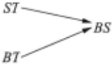
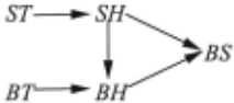
This causal model does not distinguish between Suzy and Billy's rocks hitting the bottle simultaneously and Suzy's rock hitting first. A more sophisticated model might also in clude variables SHand BH, for Suzy's rock hits the bottle and Billy's rock hits the bottle. Clearly BS is 1 iff one of B H and BT is 1. However, now, S H is 1 if ST is 1, and BH = 1 if BH = 1 and SH = 0. Thus, Billy's throw hits if Billy throws and Suzy's rock doesn't hit. This model is de scribed by the following graph, where we implicitly assume a context where Suzy throws first, so there is an edge from S H to BH, but not one in the other direction.
Given a causal model M = (S, F), a (possibly empty) vector X of variables in V, and vectors x and i1 of values for the variables in X and U, respectively, we can define a new causal model denoted M x +-x over the signature S x = ~ x - (U, V- X, Rlv-x). Formally, Mx+-x = (Sx,F +-x), where Ff +-x is obtained from Fy by setting the values of the variables in X to x. Intuitively, this is the causal model that results when the variables in X are set to x by some ex ternal action that affects only the variables in X; we do not model the action or its causes explicitly. For example, if M is the more sophisticated model for the rock-throwing example, then Msr+-o is the model where Suzy doesn't throw.
Given a signature S = (U, V, R), a formula of the form X = x, for X E V and x E R(X), is called a primitive event. A basic causal formula is one of the form [Y1 + Yl, . .. , Yk +- Yk]cp, where
- cp is a Boolean combination of primitive events;
- Y1, ... , Yk are distinct variables in V; and
- Yi E R(Y;).
Such a formula is abbreviated as [Y +- Y]cp. The special case where k = 0 is abbreviated as cp. Intuitively, [Y1 + YI , . . . , Yk +- Yk]cp says that cp holds in the counterfactual world that would arise ifY; is set to Yi, i = 1, . . . , k. A causal formula is a Boolean combination of basic causal formulas.
A causal formula cp is true or false in a causal model, given a context. We write (M, il) f= cp if cp is true in causal model M given context il. (M, il) f= [Y +- YJ(X = x) if the vari able X has value x in the unique (since we are dealing with recursive models) solution to the equations in M-y+-il in con text i1 (that is, the unique vector of values for the exogenous variables that simultaneously satisfies all equations Fi+-il, Z E V- Y, with the variables in U set toil). We extend the definition to arbitrary causal formulas in the obvious way.
3 Causality and Responsibility
3.1 Causality
We start with the definition of cause from [Halpern and Pearl, 2001a].
Definition 3.1 . We say that X =xis a cause ofcp in (M, il) if the following three conditions hold:
- ACl. (M, il) f= (X = x) A cp.
- AC2. There exist a partition (Z, W) ofV with X ~ Z and some setting ( x', w') of the variables in (X, W) such that if(M, il) f= Z = z* for Z E Z, then
- (a) (M, il) F [X +- x', w +- w']·cp. That is, chang ing ( x, w) from ( x, w) to ( x', w') changes cp from true to false.
- (b) (M,il) F= [X.._ x,w .._ w',Z' +- z*]cpforall subsets Z' of i. That is, setting w to w' should have no effect on cp as long as X has the value x, even if all the variables in an arbitrary subset of Z are set to their original values in the context il.
AC1 just says that A cannot be a cause of B unless both A and B are true, while AC3 is a minimality condition to pre vent, for example, Suzy throwing the rock and sneezing from being a cause of the bottle shattering. Eiter and Lukasiewicz 2002b showed that one consequence of AC3 is that causes can always be taken to be single conjuncts. Thus, from here on in, we talk about X = x being the cause of <p, rather than X = x being the cause. The core of this definition lies in AC2. Infor mally, the variables in Z should be thought of as describing the "active causal process" from X to <p. These are the vari ables that mediate between X and <p. AC2(a) is reminiscent of the traditional counterfactual criterion, according to which X = x is a cause of <p if change the value of X results in <p being false. However, AC2(a) is more permissive than the traditional criterion; it allows the dependence of <p on X to be tested under special structural contingencies, in which the variables W are held constant at some setting w'. AC2(b) is an attempt to counteract the "permissiveness" of AC2(a) with regard to structural contingencies. Essentially, it ensures that X alone suffices to bring about the change from <p to -.<p; setting W to ·w' merely eliminates spurious side effects that tend to mask the action of X.
To understand the role of AC2(b), consider the rock throwing example again. In the model in Figure 1, it is easy to see that both Suzy and Billy are causes of the bottle shattering. Taking Z = {ST, BS} , consider the structural contingency where Billy doesn't throw (BT = 0). Clearly [ST <--- O,BT <--- O]BS = 0 and [ST <--- 1,BT <--- O]BS = 1 both hold, so Suzy is a cause of the bottle shattering. A sym metric argument shows that Billy is also the cause.
But now consider the model described in Figure 2. It is still the case that Suzy is a cause in this model. We can take Z = { ST, SH, B S} and again consider the contingency where Billy doesn't throw. However, Billy is not a cause of the bottle shattering. For suppose that we now take Z = {BT,BH, BS} and consider the contingency where Suzy doesn't throw. Clearly AC2(a) holds, since if Billy doesn't throw (under this contingency), then the bottle doesn't shat ter. However, AC2(b) does not hold. Since BH E Z, if we set BH to 0 (it's original value), then AC2(b) requires that [BT <--- 1,ST <--- O,BH <--- O](BS = 1) hold, but it does not. Similar arguments show that no other choice of (Z, W) makes Billy's throw a cause.
3.2 Responsibility
The definition of responsibility in causal models extends the definition of causality.
Definition 3.2 The degree of responsibility of X = x for <p in (M, u), denoted dr((M, u) , (X = x), <p). is 0 if X = X is not a cause of<p in (M, u); it is 1/(k + 1) if X =xis a cause of<p in (M, u) and there exists a partition (Z, W) and setting (x', w')for which AC2 holds such that (a) k variables in w have different values in w' than they do in the context u and (b) there is no partition (Z', W') and setting (x" , w") satisfying AC2 such that only k' < k variables have different values in w" than they do the context u.
Intuitively, dr((M, u), (X = x), <p) measures the minimal number of changes that have to be made in i1 in order to make <p counterfactually depend on X . If no partition ofV to
(Z, W) makes <p counterfactually depend on (X = x), then the minimal number of changes in i1 in Definition 3.2 is taken to have cardinality oo, and thus the degree of responsibility of X = x is 0. If <p counterfactually depends on X = x, that is, changing the value of X alone falsifies <pin (M, u), then the degree of responsibility of X = x in <p is 1. In other cases the degree of responsibility is strictly between 0 and 1. Note that X = x is a cause of <p iff the degree of responsibility of X = x for <p is greater than 0.
Example 3.3 Consider the voting example from the intro duction. Suppose there are 11 voters. Voter ·i is represented by a variable Xi, i = 1, ... , 11; the outcome is represented by the variable 0, which is 1 if Mr. B wins and 0 if Mr. B wins. In the context where Mr. B wins 11-0, it is easy to check that each voter is a cause of the victory (that is X; = 1 is a cause of 0 = 1, fori = 1, ... , 11). However, the degree of responsibility of X; = 1 for is 0 = 1 is just 1/G, since at least five other voters must change their votes before chang ing X; to 0 results in 0 = 0. But now consider the context where Mr. B wins 6-5. Again, each voter who votes for Mr. B is a cause of him winning. However, now each of these voters have degree of responsibility 1. That is, if Xi = 1, changing X; to 0 is already enough to make 0 = 0; no other variables need to change.
Example 3.4 It is easy to see that Suzy's throw has degree of responsibility 1/2 for the bottle shattering both in the naive model described in Figure 1 and the "better" model of Fig ure 2 in the context where both Suzy and Billy throw. In both cases, we must consider the contingency where Billy does not throw. Although Suzy is the only cause of the bottle shat tering in the latter model, her degree of responsibility is still only 1/2, since the bottle would have shattered even if she hadn't thrown. This is a subtlety not captured by the notion of causality.
Interestingly, in a companion paper [Chockler et al., 2003] we apply our notion of responsibility to program verification. The idea is to determine the degree of responsibility of the setting of each state for the satisfaction of a specification in a given system. For example, given a specification of the form Op (eventually p is true), if p is true in only one state of the verified system, then that state has degree of responsibility 1 for the specification. On the other hand, if p is true in three states, each state only has degree of responsibility 1/3. Expe rience has shown that if there are many states with low degree of responsibility for a specification, then either the specifica tion is incomplete (perhaps p really did have to happen three times, in which case the specification should have said so), or there is a problem with the system generated by the program, since it has redundant states.
The degree of responsibility can also be used to provide a measure of the degree of fault-tolerance in a system. If a component is critical to an outcome, it will have degree of responsibility 1. To ensure fault tolerance, we need to make sure that no component has a high degree of responsibility for an outcome. Going back to the example of Op, the degree of responsibility of 1/3 for a state means that the system is robust to the simultaneous failures of at most two states.
3.3 Blame
The definitions of both causality and responsibility assume that the context and the structural equations are given; there is no uncertainty. We are often interested in assigning a de gree of blame to an action. This assignment depends on the epistemic state of the agent before the action was performed. Intuitively, if the agent had no reason to believe that his action would result in a certain outcome, then he is not to blame for the outcome (even if in fact his action caused the outcome).
To deal with the fact that we are considering two points in time-before the action was performed and after-we add superscripts to variables. We use a superscript 0 to denote the value of the random variable before the action was performed and the superscript 1 to denote the value of the random vari able after. Thus, Y 0 = 1 denotes that the random variable Y has value 1 before the action is performed, while Y 1 = 2 denotes that it had value 1 afterwards. If c.p is a Boolean com bination of (unsuperscripted) random variables, we use c.p 0 and c.p 1 to denote the value of c.p before and after the action is performed, respectively.
There are two significant sources of uncertainty for an agent who is contemplating performing an action:
- what the true situation is; for example, a doctor may be uncertain about whether a patient has high blood pres sure.
- how the world works; for example, a doctor may be un certain about the side effects of a given medication.
In our framework, the "true situation" is determined by the context and "how the world works" is determined by the structural equations. Thus, we model an agent's uncertainty by a pair (K , Pr), where K is a set of pairs of the form (M, u), where M is a causal model and u is a context, and Pr is a probability distribution over K. Following [Halpern and Pearl, 2001b], who used such epistemic states in the defini tion of explanation, we call a pair (M, u) a situation.
Roughly speaking, the degree of blame that setting X to x has for c.p is the expected degree of responsibility of X = X for c.p, taken over the situations (M X +-x ,Y +-if' u), where ( M, u, Y f- if) E K. Our actual definition of blame is just this definition, except that, when computing the expectation, we do not count situations in K where c.p was already true or X was already x. To understand why, suppose that we are trying to compute the degree of blame of Suzy's throwing the rock for the bottle shattering. Assume that we are interested in a period in a bottle in the period between time 0 and time 1, and the bottle was actually shattered at time 1. We certainly don't want to say that Suzy's throw was to blame if Suzy didn't throw between time 0 and time 1 or if the bottle was already shattered at time 0. So suppose that Suzy does in fact throw between time 0 and time 1, and at time 0, she considers the following four situations to be equally likely:
- (M1 , u1), where the bottle was already shattered before Suzy's throw;
- (M2 , u2), where the bottle was whole before Suzy's throw, and Suzy and Billy both hit the bottle simulta neously (as described in the model in Figure 1);
- (M3, u3), where the bottle was whole before Suzy's throw, and Suzy's throw hit before Billy's throw (as de scribed in the model in Figure 2); and
- (M4, u4), where the bottle was whole before Suzy's throw, and Billy did not throw.
To compute the degree of blame assigned to Suzy's throwing the rock for the bottle shattering, we ignore (M, u1), because the bottle is already shattered in (M, u1 ) before Suzy's ac tion. The degree of responsibility of Suzy's throw for the bottle shattering is 1/2 in (Mz, uz) and (M3 , u3 ), and is 1 in (M4, ·174)· It is easy to see that the degree of blame is i. ~ + i. ~ + i. 1 = ~-
Definition 3.5 The degree of blame of setting X to x for c.p relative to epistemic state (K, Pr), denoted db(K, Pr, X f x, c.p), is L{(M,u)EIC: (M,u)l=xo,o xl\ ~<pO} dr((M, u), X 1 = x, c.p 1 ) Pr((M, ·17)).
Example 3.6 Consider again the example of the firing squad with ten excellent marksmen. Suppose that marksman 1 knows that exactly one marksman has a live bullet in his rifle. Thus, he considers 10 situations possible, depending on who has the bullet. Let Pi be his prior probability that marksman i has the live bullet. Then the degree of blame of his shot for the death is Pi· The degree of responsibility is either 1 or 0, depending on whether or not he actually had the live bullet. Thus, it is possible for the degree of responsibility to be 1 and the degree of blame to be 0 (if he ascribes probability 0 to his having the live bullet, when in fact he does), and it is possi ble for the degree of responsibility to be 0 and the degree of blame to be 1 (if he mistakenly ascribes probability 1 to his having the bullet when he in fact does not).
Example 3.7 The previous example suggests that both de gree ofblame and degree of responsibility may be relevant in a legal setting. Another issue that is relevant in legal settings is whether to consider actual epistemic state or to consider what the epistemic state should have been. The former is rel evant when considering intent. To see the relevance of the latter, consider a patient who dies as a result of being treated by a doctor with a particular drug. Assume that the patient died due to the drug's adverse side effects on people with high blood pressure and, for simplicity, that this was the only cause of death. Suppose that the doctor was not aware of the drug's adverse side effects. (Formally, this means that he does not consider possible a situation with a causal model where taking the drug causes death.) Then, relative to the doctor's actual epistemic state, the doctor's degree of blame will be 0. However, a lawyer might argue in court that the doctor should have known that treatment had adverse side effects for patients with high blood pressure (because this is well documented in the literature) and thus should have checked the patient's blood pressure. If the doctor had performed this test, he would of course have known that the patient had high blood pressure. With respect to the resulting epistemic state, the doctor's degree of blame for the death is quite high. Of course, the lawyer's job is to convince the court that the lat ter epistemic state is the appropriate one to consider when assigning degree of blame.
4 The Complexity of Computing Responsibility and Blame
In this section we present complexity results for computing the degree of responsibility and blame for general recursive models.
4.1 Complexity of responsibility
Complexity results for computing causality were presented by Eiter and Lukasiewicz 2002a; 2002b. They showed that the problem of detecting whether X = :1: is an actual cause of cp is ~f -complete for general recursive models and NP complete for binary models [Eiter and Lukasiewicz, 2002b]. (Recall that ~f is the second level of the polynomial hierar chy and that binary models are ones where all random vari ables can take on exactly two values.) There is a similar gap between the complexity of computing the degree of responsi bility and blame in general models and in binary models.
For a complexity class A, FPA[Iogn] consists of all func tions that can be computed by a polynomial-time Turing ma chine with an oracle for a problem in A, which on input x asks a total of O(log lxl) queries (cf. [Papadimitriou, 1984]). We show that computing the degree of responsibility of X = x for cp in arbitrary models is FPI:f [log nLcomplete. In [Chock ler eta!., 2003], we show that computing the degree of re sponsibility in binary models is FPNP[logn]_complete.
Since there are no known natural FPI:f [log n] -complete problems, the first step in showing that computing the de gree of responsibility is FPI:f [log nLcomplete is to define an FPE:f[log n)_complete problem. We start by defining one that we call MAXQSAT2.
Recall that a quantified Boolean formula [Stockmeyer, 1977] (QBF) has the form vxax2 ... 'lj;, where X1, X2, ... are propositional variables and 'ljJ is a propositional formula. A QBF is closed if it has no free propositional variables. TQBF consists of the closed QBF formulas that are true. For example, VX3Y(X =? Y) E TQBF. As shown by Stock meyer 1977, the following problem QSAT 2 is ~f -complete:
That is, QSAT 2 is the language of all true QBFs of the form 3XVY'Ij;, 3X'<:lY'Ij;, where 'lj; is a Boolean formula in 3-CNF.
A witness f for a true closed QBF 3XVY 'lj; is an as signment f to X under which vf 'lj; is true. We define MAXQSAT 2 as the problem of computing the maximal num ber of variables in X that can be assigned 1 in a witness for 3XVY 'lj; . Formally, given a QBF <I> = 3XVY 'lj;, define MAXQSAT 2 (<I>) to be k if there exists a witness for <I> that assigns exactly k of the variables in X the value 1, and every other witness for <I> assigns at most k' ~ k variables in X the value 1. If <I>~ QSAT2, then MAXQSAT2(<I>) = -1.
The proof of Theorem 4.1 shows explicitly how to reduce the computation of any FPI:f[Iogn] problem to MAXQSAT2. Given a polynomial-time Turing machine M with oracle in
~f that on an input of size n makes O(log n) oracles queries, we construct a formula <I> = 3XVY cp, where 'lj; is a Boolean formula in 3-CNF such that given MAXQSAT 2 (<I>) we can compute the output of M in polynomial time. Essentially, the formula cp describes the output of M for all possible se quences of answers for oracle queries and MAXQSAT 2 (<I>) gives the correct sequence of answers. Since the total number of oracle queries is O(log n ), the number of all possible se quences of answers is polynomial in the size of the input, and thus the size of <I> is also polynomial in the size of the input. The construction is somewhat complicated; see the full paper for details.
Similarly to MAXQSAT 2, we define MINQSAT2(::JXVY'Ij;) to be the minimum number of variables in X that can be assigned 1 in a witness for 3XVY'Ij; if there is such a witness, and lXI + 1 otherwise. It is easy to see that MINQSAT 2 has the same complexity as MAXQSAT 2, since
where ( 'lj;) is obtained from 'lj; by replacing each propositional variable X E X with its negation.
Using a reduction from MINQSAT 2, we can prove the de sired complexity result.
Theorem 4.2 The degree of responsibility is FPI:f[logn]_ complete for general recursive causal models.
Proof: Due to lack of space, we present the proof here in a somewhat abridged form. Membership in FPI:f[Iogn] can be proved using an argument similar to the one used in [ Chockler et a/., 2003] to prove membership of the degree of responsi bility for binary causal models in FPNP[log n].
The proof that computing the degree of responsibility is FPI:fllog n]_hard essentially follows from an argument in [Eiter and Lukasiewicz, 2002a] showing that QSAT 2 can be reduced to the problem of detecting causality. In fact, their ar gument actually provides a reduction from MINQSAT 2 to the degree of responsibility. Given a QBF of the form 3XVY 'lj;, Eiter and Lukasiewicz construct a causal model M whose en dogenous variables include X, Y, and a fresh variable X *. They consider a context u in which all variables in X get the value 0. They show that VX3Y'Ij; is true iff X* = 0 is a cause of 'lj; in (M, u). If X* = 0 is indeed a cause, then the set W in AC2 must be a subset of X. That is, if there is a partition (W, Z) and a setting (x', uj') satisfying AC2 showing that X* = 0 is a cause of 'lj;, then W must be a subset of X. Moreover, the variables in W that change value from 0 to 1 in w' are precisely those such that an as signment f that assigns 1 to just those variables makes VZ·IjJ true. It then easily follows that MINQSAT2(3XVY'Ij;) = i < lXI + 1 iff dr((M, u), X* = 0, ?j;) = 1/ (i + 1), and MINQSAT2(3XVY?j;) lXI + 1 iff dr((M, u) , X* = 0,'1/J) = 0. 0
4.2 Complexity of blame
Given an epistemic state (K, Pr), where K consists of N pos sible situations, each with at most n random variables, the straightforward way to compute db(K , Pr, X <-- x, t.p ) is by computing dr((M, 11) ,X 1 = x,t.p 1 ) for each (M, 11) E K such that ( M, ·17) f= X 0 =f. :r; 1\ --.t.p 0 , and then computing the expected degree of responsibility with respect to these situa tions, as in Definition 3.5 , Recall that the degree of respon sibility in each model is determined by using a binary search thus uses O(log n) queries in each model in K. Since the number of models is N, we get a polynomial time algorithm with N log n oracle queries. The type of oracle depends on whether the models are binary or generaL For binary models it is enough to have an NP oracle, whereas for general mod els we need a Ef -oracle. We do not have a matching lower bound but, as we show in the full paper, any binary-search style algorithm for computing the degree of blame requires 0( N log n) oracle queries, for N = o( n),
Acknowledgment We thank Michael Ben-Or and Orna Kupferman for helpful discussions.
@inproceedings{ijcai2003p21,
  title     = {Responsibility and Blame: A Structural-Model Approach},
  author    = {Chockler, Hana and Halpern, Joseph Y.},
  booktitle = {Proceedings of the Eighteenth International Joint Conference on
               Artificial Intelligence, {IJCAI-03}},
  publisher = {International Joint Conferences on Artificial Intelligence},
  editor    = {Georg Gottlob and Toby Walsh},
  pages     = {147--152},
  year      = {2003},
  url       = {https://ijcai.org/proceedings/2003/21},
}
TY - CPAPER TI - Responsibility and Blame: A Structural-Model Approach AU - Chockler, Hana AU - Halpern, Joseph Y. T2 - Proceedings of the Eighteenth International Joint Conference on Artificial Intelligence, IJCAI-03 PB - International Joint Conferences on Artificial Intelligence PY - 2003 SP - 147 EP - 152 UR - https://ijcai.org/proceedings/2003/21 ER -Copied
Machine-readable versions of this paper, for tools and AI agents:





