DP-SLAM: Fast, Robust Simultaneous Localization and Mapping Without Predetermined Landmarks

1 Introduction

The availability of relatively inexpensive laser range finders and the development of particle filter based algorithms have led to great strides in recent years on the problem of robot localization - determining a robot's position given a known map [Fox et al., 1999]. Initially, the maps used for these methods were constructed by hand. However, the accuracy of the laser suggests its use for map-making as well as lo­ calization. Potential applications for accurate map-making would include search and rescue operations, as well as space, underwater and subterranean exploration.

Even with an accurate laser range finder, map-making presents a difficult challenge: A precise position estimate is required to make consistent updates to the the map, but a good map is required for reliable localization. The challenge of si­ multaneous localization and mapping (SLAM) is that of pro­ ducing accurate maps in real time, based on a single pass over the sensor data, without an off line correction phase. Straight­ forward approaches that localize the robot based upon a par­ tial map and then update the map based upon the maximum likelihood position of the robot tend to produce maps with er­ rors that accumulate over time. When the robot closes a physicalloop in the environment, serious misalignment errors can result.

The EM algorithm provides a very principled approach to the problem, but it involves an expensive off-line alignment phase [Burgard et al., 1999]. There exist heuristic approaches to this problem that fall short of full EM 1 , but they are not a complete solution and they require additional passes over the sensor data [Thrun, 2001]. Scan matching can produce good maps [Lu and Milios, 1997; Gutmann and Konolige, 2000] from laser range finder data, but such approaches typically must explicitly look for and require additional effort to close loops. In varying degrees, these approaches can be viewed as partially separating the localization and mapping components of SLAM.

The FastSLAM algorithm [Montemerlo et al., 2002], which does not require explicit loop-closing heuristics, is a recent SLAM approach which has made great progress in the field. FastSLAM follows a proposal by Murphy [Mur­ phy, 1999] using a Rao-Blackwellized particle filter to sam­ ple robot poses and track the position of a fixed number of predetermined landmarks using a Kalman filter. (The land­ mark positions are conditionally independent given the robot pose.) This method mitigates some of the challenges in map­ ping at the expense of some challenges in landmark selection and identification. The latter can involve a fairly complicated data association problem, although recent progress has been made in addressing this [Montemerlo and Thrun, 2002].

We present a novel, laser range finder based algorithm called DP-SLAM that, like FastSLAM, exploits the condi­ tional independences noted by Murphy. However, our algo­ rithm is purely laser based and makes no landmark assump­ tions. We avoid the data association problem by storing mul­ tiple detailed maps instead of sparse landmarks, thereby sub­ suming association with localization. Our algorithm uses a particle filter to represent both robot poses and possible map configurations. Using a new map representation, which we call distributed particle (DP) mapping, we are able to main­ tain and update hundreds or thousands of candidate maps and robot poses in real time as the robot moves through the en­ vironment. The worst-case complexity of our algorithm per laser sweep is log-quadratic in the number of particles we maintain and linear in the area swept out by the laser. How­ ever, in practice our run time is usually much less. Our tech­ nique makes essentially no assumptions about the environ­ ment yet it is accurate enough to close loops of 60m in length with crisp, perpendicular edges on corridors and minimal or no misalignment errors. This accuracy is achieved throughout the mapping process, without a need for explicit algorithms to correct the loop as temporally distant observations begin to overlap. In fact, DP-SLAM could be further complimented by inclusion of existing algorithms for closing loops, though the addition may be unnecessary if a sufficient number of par­ ticles is used.

1 This approach is heuristic because it does not maintain a joint probability distribution over maps and poses.

2 Particle Filters for Localization and Mapping

A particle filter is a simulation-based method of tracking a system with partially observable state. We briefly review par­ ticle filters here, but refer the reader to excellent overviews of this topic [Doucet et a!., 200 1] and its application to robotics [Thrun, 2000] for a more complete discussion.

A particle filter maintains a weighted (and normalized) set of sampled states, S = { s 1 ... s111 }, called particles. At each step, upon observing an observation o (or vector of observa­ tions), the particle filter:

1. Samples m new states S' = { s~ ... s:n} from S with replacement.
2. Propagates each new state through a Markovian transi­ tion (or simulation) model: P(s"ls'). This entails sam­ pling a new state from the conditional distribution over next states given the sampled previous state.
3. Weighs each new state according to a Markovian obser­ vation model : P(ols")
4. Normalizes the weights for the new set of states

Particle filters are easy to implement have been used to track multimodal distributions for many practical prob­ lems [Doucet eta!., 200 I].

2.1 Particle Filters for Localization

A particle filter is a natural approach to the localization prob­ lem, where the robot pose is the hidden state to be tracked. The state transition is the robot's movement and the observa­ tions are the robot's sensor readings, all of which are noisy.

The change of the state over time is handled by a mo­ tion model. Usually, the motion indicated by the odometry is taken as the basis for the motion model, as it is a reliable measure of the amount that the wheels have turned. However, odometry is a notoriously inaccurate measure of actual robot motion, even in the best of environments. The slip and shift of the robot's wheels, and unevenness in the terrain can com­ bine to give significant errors which will quickly accumulate. A motion model differs across robots and types of terrain, but generally consists of a linear shift, to account for systematic errors and Gaussian noise. Thus, for odometer changes of x, y and B, a particle filter applies the error model and obtains, for particle i ,

The a and b terms are linear correction to account for consis­ tent errors in motion. The function N(O, a) returns random noise from a normal distribution with mean 0 and standard deviation a, which is derived experimentally and may depend upon the magnitudes of X, y, and 8.

After simulation, we need to weight the particles based on the robot's current observations of the environment. For pure localization, the robot stores a map in memory. The position described by each particle corresponds to a distinct point and orientation in the map. Therefore, it is relatively simple to de­ termine what values the sensors should return, given the pose within the map. The standard assumption is that sensor errors are normally distributed. Thus, if the first obstruction in the map along a line traced by a laser cast is at distance d and the reported distance is d', the probability density of observing discrepancy J = d' - d, is normally distributed with mean 0. For our experiments we assumed a standard deviation in laser measurements of Scm. Given the model and pose, each sen­ sor reading is correctly treated as an independent observation [Murphy, 1999]. The total posterior for particle i is then

where Jik is the difference between the expected and per­ ceived distances for sensor (laser cast) k and particle i.

2.2 Particle Filters for SLAM

Some approaches for SLAM using particle filters attempt to maintain a single map with multiple robot poses [Thrun, 200 1], an approach that we avoid because it leads to errors that accumulate over time. The basic problem is that the hid­ den state is actually both the robot pose and the map itself. An important consequence of this problem is that all observations are no longer compared to a single map, which is presumed to be correct. Instead, the observations are compared against an incomplete and possibly incorrect map, identified with the particle in question. The map itself is created by the accu­ mulation of observations of the environment and estimates of robot positions.

In principle, this "solves" the SLAM problem. In prac­ tice, it replaces a conceptual problem with an algorithmic one. Particles with errors in robot position estimates will make er­ roneous additions to their maps. An error in the map will then, in tum, cause another error in localization in the next step, and these inaccuracies can quickly compound. Thus, the number of particles required for SLAM is typically more than that required for localization since the price of accumu­ lated errors is much higher. Note that in pure localization, small errors in position estimation can be absorbed as part of the noise in the motion model.

The algorithmic problem becomes one of efficiently main­ taining a large enough set of particles to obtain robust perfor­ mance, where each particle is not merely a robot pose, but a pose and map. Since maps are not light weight data struc­ tures, maintaining the hundreds or thousands of such maps poses a serious challenge. One reasonable approach to tam­ ing this problem is to assume that the uncertainty in the map can be represented in a simple parametric form. This is essen­ tially the approach taken by FastSLAM, for which the map is a Kalman filter over a set of landmark positions. This is cer­ tainly the right thing to do if one is given a set of landmarks that can be quickly and unambiguously identified. We will show that this strong assumption is not required: By using raw laser data, combined with an occupancy grid and efficient data structures, we can handle a large number of candidate maps and poses efficiently, achieving robust performance.

3 DP-SLAM

In this section we motivate and present the main technical contribution of the DP-SLAM algorithm. DP-SLAM imple­ ments what is essentially a simple particle filter over maps and robot poses. However, it uses a technique called dis­ tributed particle mapping (DP-Mapping), which enables it to maintain a large number of maps very efficiently.

3.1 Naive SLAM

When using a particle filter for SLAM, each particle corre­ sponds to a specified trajectory through the environment and has a specific map associated with it. When a particle is re­ sampled, the entire map itself is treated as part of the hidden state that is being tracked and is copied over to the new parti­ cle. If the map is an occupancy grid of size M and P particles are maintained by the particle filter, then ignoring the cost of localization, O(M P) operations must be performed merely copying maps. For a number of particles sufficient to achieve precise localization in a reasonably sized environment, the naive approach would require gigabytes worth of data move­ ment per update 2 .

3.2 Distributed Particle Mapping

By now the astute reader has most likely observed that the naive approach is doing too much work. To make this clearer, we will introduce the notion of a particle ancestry. When a particle is sampled at iteration i to produce a successor parti­ cle at iteration i + 1, we call the generation i particle a parent and the generation i + 1 particle a child. Two children with the same parent are siblings. From here, the concept of a par­ ticle ancestry extends naturally. Suppose the laser sweeps out an area of size A « M and consider two siblings, 8 1 and 8 2 . Each sibling will correspond to a different robot pose and will make at most A updates to the map it inherits from its parent. Thus, 8 1 and 8 2 can differ in at most A map positions.

When the problem is presented in this manner, the natural reaction from most computer scientists is to propose record­ ing the "diff" between maps, i.e, recording a list of changes that each particle makes to its parent's map. While this would solve the problem of making efficient map updates, it would create a bad computational problem for localization: Trac­ ing a line though the map to look for an obstacle would re­ quire working through the current particle's entire ancestry and consulting the stored list of differences for each particle in the ancestry. The complexity of this operation would be linear in the number of iterations of the particle filter. The challenge is, therefore, to provide data structures that permit efficient updates to the map and efficient localization queries with time complexity that is independent of the number of iterations of the particle filter. We call our solution to this problem Distributed Particle Mapping or DP-Mapping, and we explain it in terms of the two data structures that are main­ tained: the ancestry tree and the map itself.

2 In addition to the theoretical analysis, anecdotal comments made by researchers in this area reinforce the impracticality of this approach.

Maintaining the particle ancestry tree

The basic idea of the particle ancestry tree is fairly straight­ forward. The tree itself is rooted with an initial particle, of which all other particles are progeny. Each particle maintains a pointer to its parent and is assigned a unique numerical ID. Finally each particle maintains a list of grid squares that it has updated.

The details of how we will use the ancestry tree for local­ ization are described in the subsequent section. In this section we focus on the maintenance of the ancestry tree, specifically on making certain that the tree has bounded size regardless of the number of iterations of the particle filter.

We maintain a bounded size tree by pruning away unnec­ essary nodes. First, note that certain particles may not have children and can simply be removed from the tree. Of course, the removal of such a particle may leave its parent without children as well, and we can recursively prune away dead branches of the tree. After pruning, it is obvious that the only particles which are stored in our ancestry tree are exactly those particles which are ancestors of the current generation of particles.

This is still somewhat more information than we need to remember. If a particle has only one child in our ancestry tree, we can essentially remove it, by collapsing that branch of the tree. This has the effect of merging the parent's and child's updates to the map, a process described in the subse­ quent section. By applying this process to the entire tree after pruning, we obtain a minimal ancestry tree, which has several desirable and easily provable properties:

Proposition 3.1 Independent of the number of iterations of particle filtering, a minimal ancestry tree of P particles

1. has exactly P leaves,
2. has branching factor of at least 2, and
3. has depth no more than P.

Map representation

The challenge for our map representation is to devise a data structure that permits efficient updates and efficient localiza­ tion. The naive approach of a complete map for each parti­ cle is inefficient, while the somewhat less naive approach of simply maintaining history of each particle's updates is also inefficient because it introduces a dependency on the number of iterations of the particle filter.

Our solution to the map representation problem is to asso­ ciate particles with maps, instead of associating maps with particles. DP-mapping maintains just a single occupancy grid. (The particles are distributed over the map.) Unlike a traditional occupancy grid, each grid square stores a balanced tree, such as a red-black tree. The tree is keyed on the IDs of the particles that have made changes to the occupancy of the square.

The grid is initialized as a matrix of empty trees. When a particle makes an observation about a grid square it inserts its ID and the observation into the associated tree. Notice that this method of recording maps actually allows each particle to behave as if it has its own map. To check the value of a grid square, the particle checks each of its ancestors to find the most recent one that made an observation for that square. If no ancestor made an entry, then the particle can treat this position as being unknown.

We can now describe the effects of collapsing an ancestor with a single child in the ancestry tree more precisely: First, the set of squares updated by the child is merged into the par­ ent's set. Second, for each square visited by the child, we change the ID key stored in the balanced tree to match that of the parent. (If both the child and parent have made an update to the same square, the parent's update is replaced with the child's.) The child is then removed from the tree and the par­ ent's grandchildren become its direct children. Note that this ensures that the number of items stored in the balanced tree at each grid square is O(P).

3.3 Computational Complexity

The one nice thing about the naive approach of keeping a complete map for each particle is the simplicity: If we ig­ nore the cost of block copying maps, lookups and changes to the map can all be done in constant time. In these areas, distributed particle mapping may initially seem less efficient. However, we can show that DP maps are in fact asymptoti­ cally superior to the naive approach.

Lookup on a DP-map requires a comparison between the ancestry of a particle with the balanced tree at that grid square. Let D be the depth of the ancestry tree, and thus is the maximum length of a particle's ancestry. Strictly speak­ ing, as the ancestry tree is not guaranteed to be balanced, D can be O(P). However, in practice, this is almost never the case, and we have found D ~ O(lgP), as the nature of parti­ cle resampling lends to very balanced ancestry trees. (Please see the discussion in the following section for more detail on this point.) Therefore, we can complete our lookup after just D accesses to the balanced tree. Since the balanced tree itself can hold at most P entries, and a single search takes O(lgP) time. Accessing a specific grid square in the map can there­ fore be done in O(DlgP) time.

For localization, each particle will need to make O(A) ac­ cesses to the map. As each particle needs to access the en­ tire observed space for its own map, we need O(AP) ac­ cesses, giving localization with DP-maps a complexity of O(ADPlgP).

To complete the analysis we must handle two remaining details: The cost of inserting new information into the map, and the cost of maintaining the ancestry tree. Since we use a balanced tree for each grid square, insertions and deletions on our map both take O(lgP) per entry. Each particle can make at most O(A) new entries, which in tum will only need to be removed once. Thus the procedure of adding new entries can be accomplished in O(ADlgP) per particle, or O(AD PlgP)

total and the cost of deleting childless particles will be amor­ tized as O(ADPlgP).

It remains to be shown that the housekeeping required to maintain the ancestry tree has reasonable cost. Specifically, we need to show that the cost of collapsing childless ancestry tree nodes does not exceed O(ADPlgP). This may not be obvious at first, since successive collapsing operations can make the set of updated squares for a node in the ancestry tree as large as the entire map. We now argue that the amortized cost of these changes will be O(ADPlgP) . First, consider the cost of merging the child's list of modified squares into the parent's list. If the child has modified n squares, we must perform O(nlgP) operations (n balanced tree queries on the parent's key) to check the child's entries against the parent's for duplicates.

The final step that is required consists of updating the ID for all of the child's map entries. This is accomplished by deleting the old ID, and inserting a new copy of it, with the parent's ID. The cost of this is again O(nlgP). Consider that each map entry stored in the particle ancestry tree has a po­ tential of D steps that it can be collapsed, since D is the total number of nodes between its initial position and the root, and no new nodes will ever be added in between. At each itera­ tion, P particles each create A new map entries with potential D. Thus the total potential at each iteration is O(ADPlgP).

The computational complexity of DP-SLAM can be sum­ marized as follows :

Proposition 3.2 For a particle filter that maintains P parti· cles, laser that sweeps out A grid squares, and an ancestry tree of depth D, DP-SLAM requires:

• O(ADPlgP) operations for localization arising from:
• P particles checking A grid squares
• A lookup cost ofO(DlgP) per grid square
• O(APlgP) operations to insert new data into the tree, arising from:
• P particles inserting information at A grid squares
• Insertion cost ofO(lgP) per new piece of information
• Ancestry tree maintenance with amortized cost O(ADPlgP) arising from
• A cost ofO(lgP) to remove an observation or move it up one level in the ancestry tree
• A maximum potential of AD P introduced at each iteration.

3.4 Complexity Comparison

Our analysis shows that the amortized complexity of DP-SLAM is O(ADPlgP), which can be as large as O(AP 2 lgP). For the naive approach, each map is repre­ sented explicitly, so lookups can be done in constant time per grid square. The localization step thus takes only O(AP). Without the need for updates to an ancestry tree, map updates can likewise be done in O(AP) time. However, the main bulk of computation lies in the need to copy over an entire map for each particle, which will require O(M P) time, where M is the size of the map. Since typically M » A, this obviously is the dominant term in the computation.

DP-SLAM will be advantageous when ADlgP < M. Even in the worst case where D approaches P, there will still be a benefit. For a high resolution occupancy grid, M will be quite large since it grows quadratically with the linear mea­ sure of the environment and would grow cubically if we we consider height. Moreover, A, will be a tiny fraction of M. The size of DlgP will, of course, depend upon the environ­ mental features and the sampling rate of the data. It is impor­ tant to note that since the time complexity of our algorithm does not depend directly on the size of the map, there will necessarily exist environments for which DP-SLAM is vastly superior to the naive approach since the naive approach will require block copying an amount of data will exceed physical memory.

In our initial experiments, we have observed that P was surprisingly small, suggesting that in practice the advantage of DP-SLAM is much greater than the worst-case analysis suggests. For some problems the point at which it is advan­ tageous to use DP-SLAM may be closer to Alg 2 P < M. This phenomenon is discussed in more detail in the subse­ quent section.

4 Empirical Results

We implemented and deployed the DP-SLAM algorithm on a real robot using data collected from the second floor of our computer science building. In our initial implementation our map representation is a binary occupancy grid. When a par­ ticle detects an obstruction, the corresponding point in the occupancy grid is marked as fully occupied and it remains occupied for all successors of the particle. (A probabilistic approach that updates the grid is a natural avenue for future work.)

On a fast PC (2.4 GHz Pentium 4), the run time of DP­ SLAM is close to that of the data collection time, so the algo­ rithm could have been run in real time for our test domains. In practice, however, we collected our data in a log file using the relatively slow computer on our robot, and processed the data later using a faster machine. To speed things up, we also implemented a novel particle culling technique to avoid fully evaluating the posterior for bad particles that are unlikely to be resampled. This works by dividing the sensor readings for each particle into k disjoint, evenly distributed subsets. The posterior for the particles is computed in k passes, where pass i evaluates the contribution from subset i. At the end of each pass, particles with significantly lower (partially evaluated) posterior in comparison to the others are assigned 0 proba­ bility and removed from further consideration. We also set a hard threshold on the number of particles we allowed the al­ gorithm to keep after culling. Typically, this was set to the top 10% of the total number of particles considered. In practice, this cutoff was almost never used since culling effectively re­ moved at least 90% of the particles that were proposed. A value if k = 6 gave us a speedup of approximately 6x.

For the results we present, it is important to emphasize that our algorithm knows absolutely nothing about the environ­ ment or the existence of loops. No assumptions about the environment are made, and no attempt is made to smooth over errors in the map when loops are closed. The precision in our maps results directly from the robustness of maintaining multiple maps.

4.1 Robot and Robot Model

The robot we used for testing DP-SLAM is an iRobot ATRV Jr. equipped with a SICK laser range finder attached to the front of the robot at a height of 7cm. Readings are made across 180°, spaced one degree apart, with an effective dis­ tance of up to 8m. The error in distance readings is typically less than 5mm.

Odometric readings from the ATRV Jr.'s shaft encoders are unreliable, particularly when turning. Our motion model as­ sumes errors are distributed in a Gaussian manner, with a standard deviation of25% in lateral motion and 50% in turns. Turns are quasi-holonomic, performed by skid steering. We obtained our motion model using an automated calibration procedure that worked by positioning the robot against a smooth wall and comparing odometry data with the move­ ment inferred from the laser readings.

4.2 Test Domain(s) and Map(s)

We tested the algorithm on a loop of hallway approximately 16m by 14m. A new set of observations was recorded af­ ter each 20cm motion (approximately). The maps were con­ structed with a resolution of 3cm per grid square, providing a very high resolution cross section of the world at a height of 7cm from the floor.

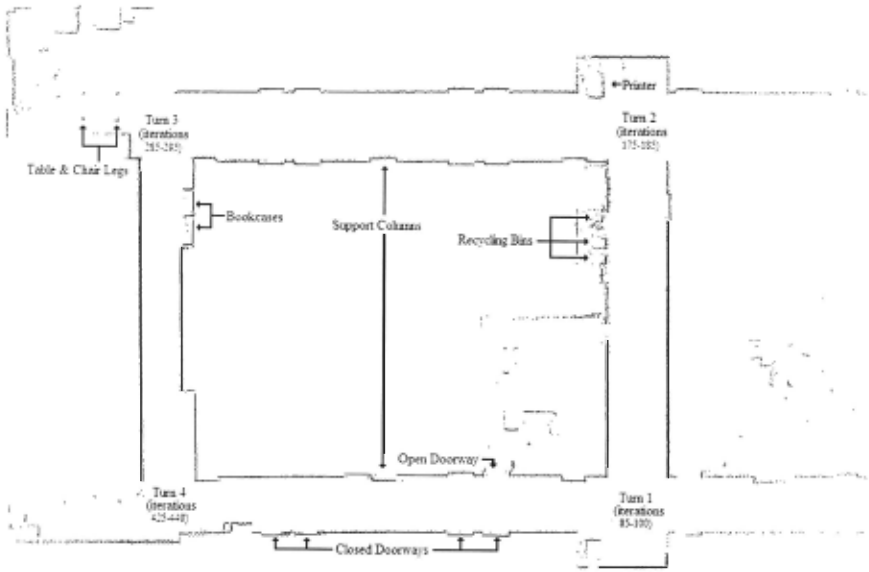
Figure 1 shows the highest probability map generated after the completion of one such loop using 9000 particles 3 . In this test, the robot began in the middle of the bottom hallway and continued counterclockwise through the rest of the map, returning to the starting point.

This example demonstrates the accuracy of DP-SLAM when completing a long loop, one of the more difficult tasks for SLAM algorithms. After traveling 60m, the robot is once again able to observe the same section of hallway in which it started. At that point, any accumulated error will readily be­ come apparent, as it will lead to obvious misalignments in the corridor. As the figure shows, the loop was closed perfectly, with no discernible misalignment.

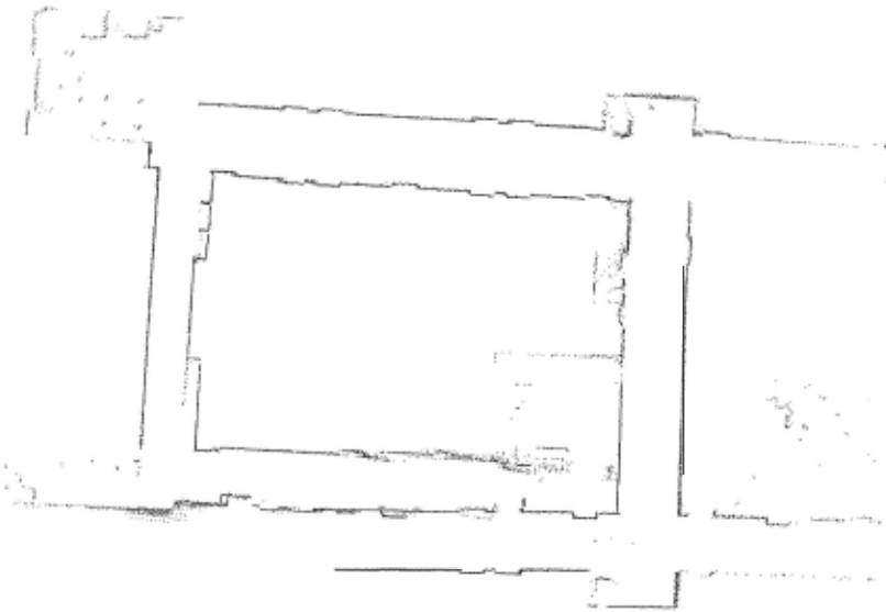
To underscore the advantages of maintaining multiple maps, we have included the results obtained when using a single map and the same number of particles. Figure 2 shows the result of processing the same sensor log file by generating 9000 particles at each time step, keeping the single particle with the highest posterior, and updating the map based upon the robot's pose in this particle. There is a considerable mis­ alignment error where the loop is closed at the top of the map.

Larger, annotated versions of the maps shown here, as well as maps generated from different sensor logs, will be avail­ able at http: I /www. cs .duke. edu;-parr/dpslam/.

3 In an earlier version of this paper, we presented a map produced with 1000 particles based upon a different sensor log file. The run shown here covers the same area, but has less reliable odometry, probably due to weaker battery, and is more illustrative of the bene­ fits of DP-SLAM.

4.3 Coalescence

In our sample domain (the second floor of the Duke Univer­ sity Department of Computer Science), we have found that DP-SLAM produces very shallow ancestry trees due to a phe­ nomenon we refer to as coalescence. Over a number itera­ tions of the particle filter, nearly all of the particles will have a common ancestor particle in the not-too-distant past. This point of coalescence, or common ancestry, varies over time, and is sensitive to the environment. Observations made on our empirical results indicate that while this number peaked during events of higher uncertainty, coalescence was often as recent as 20 generations in the past, and never exceeded 90. This means that beyond about 20 steps in the past, ev­ ery particle has an identical map. The fact that we can close loops so precisely while maintaining relatively shallow coa­ lescence points suggests that we are able to maintain distri­ butions over map regions long enough to resolve ambiguities, but not longer than is needed. While the phenomenon de­ serves more careful study, our initial impression is that by the time a region has passed outside of the robot's field of view, it has been scanned enough times by the laser that there is only a single hypothesis that is consistent with the accumulated observations.

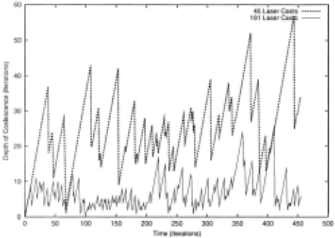
Additional experiments were run to show the relationship between coalescence and uncertainty, as well as the ability of DP-SLAM to automatically preserve more information when required. We considered two different scenarios: the origi­ nal DP-SLAM algorithm with the same sensor data used to generate Figure 1, and a handicapped version of DP-SLAM run on the same sensor log, but with three out of every four laser casts ignored at each iteration. The handicapped version required 30, 000 particles to produce good maps.

To study the effects of uncertainty on coalescence, we ran both algorithms with the same number of particles and then compared the coalescence points. The results in Figure 3 show how the two versions of DP-SLAM performed on the same sensor log with the same number of particles. The de­ crease in observational information for the handicapped ver­ sion of DP- SLAM makes it more difficult for the robot to be certain about its position. This is reflected in the higher peaks in the graph, and the less recent point of coalescence overall.

In both cases, strong correlation can be seen between the higher peaks in this graph and the turns that the robot took in the map. (Note the iteration number annotations at the turns in Figure 1.) This is because odometry is particularly unreli­ able during skid turns and the robot has greater difficulty lo­ calizing. The points at which our turns occur in our office en­ vironment also tend to produce more ambiguous sensor data since turns are typically in open areas where the laser scans will be more widely spaced. Other peaks can be mapped to areas of clutter in the map, such as the recycling bins.

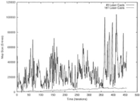
Figure 4 was created from the same two experiments, and tracks the amount of memory used over time, as measured by the total number of leaves in the balanced trees stored in our occupancy grid. Since no leaves are stored for empty space and our maps are essentially two one-dimensional sur­ faces, the amount of memory required for leaves should grow roughly linearly over time. The peaks corresponding to the turns in the map are even more pronounced for the handi­ capped version of DP-SLAM in this graph, indicating that un­ der conditions of greater uncertainty, the ancestry tree grows in width as well as depth.

Of course, shallow coalescence may not occur and may not even be desirable in all environments, but it has signifi­ cant implications for the efficiency of the algorithm when it does occur. It implies D « P, making our O(ADPlgP) bound closer to O(APlg 2 P) in practice. Moreover, we get maximum benefit from the compactness of our map repre­ sentation. As the particles coalesce, irrelevant entries are re­ moved. Thus all areas in the map that were observed before the point of coalescence contain only one entry in their list. Similarly, those areas which have not been observed by any particle yet have no entries in their list. If we can assume that the depth of coalescence is bounded by some reasonable con­ stant C, then all map squares but those that have been altered prior the point of coalescence can be thought of as requiring a constant amount of storage. This means that the total space required to store the map tends to be close to O(M + APC) in practice, not the theoretical worst case of 0( M P).

A sceptic may wonder if coalescence is indeed a desirable thing since it may imply a loss of information. If the algo­ rithm maintains only a limited window of uncertainty, how can it be expected to close large loops, which would seem to require maintaining uncertainty over map entries for arbi­ trarily long durations? The simple answer is that coalescence is desirable when it is warranted by the data and undesirable when the accumulation of sensor data is insufficient to re­ solve ambiguities. In fact, coalescence is a direct product of the amount of uncertainty still present in the observations. Our algorithm is both able to maintain ambiguity for arbi­ trary time periods and benefit from coalescence when it is warranted, so there is nothing negative about the fact that we have observed this phenomenon in our experiments.

Of course, since we are representing a complicated distri­ bution with a finite number of samples, there is always a dan­ ger that the low probability "tails" of the distribution will be lost if too few particles are used. This would result in pre­ mature coalescence due to failure to resample a potentially useful and correct map. There will certainly be some envi­ ronments, typically those with very sparse sensor data, where it will be difficult to avoid premature coalescence without an excessive number of particles. In situations with sparse data, a parametric representation of uncertainty over land­ marks may be more tractable and more appropriate.

5 Conclusion and Future Work

We have presented a novel particle-filter based algorithm for simultaneous localization and mapping. Using very efficient data structures, this algorithm is able to maintain thousands of maps in real time, providing robust and highly accurate map­ ping. The algorithm does not assume the presence of pre­ determined landmarks or assume away the data association problem created by the use of landmarks. Our algorithm has been deployed on a real robot, where it has produced highly detailed maps of an office environment.

We believe that this is the first time this level of accuracy has been achieved for the type of data we consider using an algorithm that does not explicitly attempt to close loops and that has no domain specific knowledge. Nevertheless, our al­ gorithm does have some limitations. Most reasonably priced laser range finders scan at a fixed height, giving us an incom­ plete view of the environment. Our current map representa­ tion is very simplistic - a grid where each cell is presumed to be completely clear or completely opaque to the laser. This obviously creates discretization errors at the edges of objects and confusion for very small objects. Our small cell size re­ duces this problem, but does not eliminate it entirely. For example, power cords hanging off of the edge of desks tend to introduce localization errors and increase the number of particles needed to get robust performance.

There is a logical inconsistency in the way we treat the laser data. When we add new information to the map, we treat the laser like a deterministic device, but when we local­ ize. we treat it like a noisy device with a standard deviation in measurement that can span several grid squares. Exaggerated error models like this are common in many real-world appli­ cations of statistical models, where additional noise is added to one part of the model to compensation for unmodeled noise in other parts. Nevertheless, in future work we would like to develop a more comprehensive error model and a principled scheme for updating the map that handles partially or tran­ siently occupied grid squares. Naturally, we would like to consider other map representation methods too.

The most important future direction for this work is to in­ corporate less reliable sensors as such video or sonar to con­ struct a more comprehensive, three-dimensional view of the environment.

Acknowledgments

We are very grateful to Sebastian Thrun for critical feedback and encouragement for this line of research.We also thank Tammy Bailey, Dieter Fox, Carlos Guestrin, Dirk Haehnel, Mark Paskin, and Carlo Tomasi for helpful feedback and comments.