
Consistent, Convergent, and Constant-Time SLAM
Proceedings of the Eighteenth International Joint Conference on Artificial Intelligence. Pages 1143-1149.
© 2003 International Joint Conferences on Artificial Intelligence
Abstract
This paper presents a new efficient algorithm for simultaneous localization and mapping (SLAM), using multiple overlapping submaps, each built with respect to a local frame of reference defined by one of the features in the submap. The global position of each submap is estimated using information from other submaps in an efficient, provably consistent manner. For situations where the mobile robot is able to make repeated visits to all regions of the environment, the method achieves convergence to a near-optimal result with 0(1) time complexity while maintaining consistent error bounds. Simulation results demonstrate the ability of the technique to converge to errors that are only slightly greater than the full solution, while maintaining consistency.
- [Bosse eta /. , 2003] M. Bosse, P. Newman, J. Leonard, M. Soika, W. Feiten, and S. Teller. An atlas framework for scalable mapping. In Proc. IEEE Int. Con[ Robotics and Automation, 2003.
- [Choset and Nagatani, 2001] H. Choset and K. Nagatani. Topological simultaneous localization and mapping (SLAM): toward exact localization without explicit local• ization. IEEE Transactions on Robotic and Automation, 17(2): 125-1 37, April 200 I.
- [Dissanayake eta/. , 2001] M. W. M. G. Dissanayake, P. Newman, H. F. Durrant- Whyte, S. Clark, and M. Csorba. A solution to the simultaneous localization and map building (SLAM) problem. IEEE Transactions on Robotic and Automation, 17(3):229-24 1, June 2001.
- [Guivant and Nebot, 2001] J. Guivant and E. Nebot. Optimization of the simultane- ous localization and map building algorithm for re al time implementation. IEEE Transactions on Robotic and Automation, 17(3):242-257, June 200 I.
- [Gutmann and Konolige, 1999] J-S. Gutmann and K. Konolige. Incremental mapping of large cyclic environments. In International Symposium on Computational Intelli- gence in Robotics and Automation, I 999.
- Hahnel era/., 20021 D. Hahne!, D. Schulz, and W. Burgard. Map building wi th mobile robots in populated environments. In Proc. IEEE Int. Workshop on Intelligent Robots and Systems, 2002.
- [Julier and Uhlmann, 2001] S. J. Julier and J. K. Uhlmann. Building a Million Beacon Map. In Sensor Fusion . SPIE, 200 I.
- [Knight, 2002] J. Knight. Towards Fully Autonomous Visual Navigation. PhD thesis, University of Oxford, 2002.
- [Kuipers and Beeson, 2002] B. Kuipers and P. Beeson. Bootstrap learning for place recognition. In Proceedings of the AAAI National Conference on Artijicial llllelli- gence, Edmonton, Canada, 2002. AAAI.
- Leonard and Feder, 20001 J. J. Leonard and H. J. S. Feder. A computationally effi- cient method for large-scale concurrent mapping and localization. In D Koditschck and J. Hollerbach, editors, Robotics Research: The Ninth International Symposium, pages 169-176, Snowbird, Utah, 2000. Springer Verlag. [Montemerlo era/., 2002]
- M. Montemerlo, S. Thrun, D. Koller, and B. Wegbreit. Fast- SLAM: A factored solution to the simultaneous localization and mapping problem. In Proceedings of the AAAI National Coriference on Artijicial lnrelligence, Edmon- ton, Canada, 2002. AAAI.
- [Neira and Tard6s, 2001] J. Neira and J.D. Tard6s. Data association in stochastic map- ping using the joint compatibility test. IEEE Trans. on Robotics and Automation, 17(6):890-897, 2001.
- [Neira eta/., 2002] J. Neira, J.D. Tard6s, and J.A. Castellanos. Linear time vehicle re- location in SLAM. Technical Report RR-2002-08, Universidad de Zaragoza, Depto. de Informatica e lng. de Sistemas, Zaragoza, Spain, 2002.
- [Smither a/., 1987] R. Smith, M. Self, and P. Cheeseman. A stochastic map for un- certain spatial relationships. In 4th International Symposium on Robotics Research. MIT Press, I 987. [
- [Tard6s era/., 2002] J.D. Tard6s, J. Neira, P.M. Newman, and J.J . Leonard. Robust mapping and localization in indoor environments using sonar data. Int. J. Robotics Research, 21(4):311-330, April 2002.
- [Thrun eta/., 2002] S. Thrun, D. Koller, Z. Ghahramani, H. Durrant-Whyte, and Ng. A.Y. Simultaneous mapping and localization with sparse extended information fi l- ters. In J.-D. Boissonnat, J. Burdick, K. Goldberg, and S. Hutchi nson, editors, Proceedings of the Fifth l/1/ernationa/ Workshop on Algorithmic Foundations of Robotics, Nice, France, 2002. Forthcoming.
- Thrun, 200
- S. Thrun. A probabilistic online mapping algorithm for teams of mobile robots. Int. J. Robotics Research, 20(5):335-363, May 2001.
- [Williams era/., 2002] S. B. Williams, G. Dissanayake, and H. Durrant-Whyte . An efficient approach to the simultaneous localisation and mapping problem. In Proc. IEEE Int. Con[ Robotics and Automation, pages 406-411 , May 2002.
References were extracted automatically from the PDF and may contain errors.
Full text extracted automatically from the PDF; figures, tables and equations may differ. The PDF is the version of record.
1 Introduction
The capability of simultaneous localization and mapping (SLAM) is considered vital for the creation of long-lived autonomous mobile agents. Because of the difficulties en countered by SLAM algorithms when applied to larger envi ronments, the "map scaling" problem has been identified as one of the key issues for research in this area. In this pa per, we adopt the feature-based, state-space formulation of SLAM [Smith et al., 1987]. Recent related work in SLAM in cludes submap decomposition methods [Leonard and Feder, 2000; Guivant and Nebot, 2001; Julier and Uhlmann, 2001; Williams et at., 2002; Tard6s eta!., 2002], FastS LAM [Mon temerlo et al., 2002], sparse extended information filters (SElF's) [Thrun et al., 2002], scan-matching [Gutmann and Konolige, 1999; Thrun, 2001; Hahne) et al., 2002] and topo logical approaches [Kuipers and Beeson, 2002; Choset and Nagatani, 2001].
*This research has been funded in part by NSF Career Award BES-9733040, the MIT Sea Grant College Program under grant NA86RG0074, and the Office of Naval Research under grant N00014-97-0202.
tp_ Newman is at the Robotics Research Group, University of Oxford and J. Leonard is at the Department of Ocean Engineering at MIT, email : pnewman@robots.ox.ac.uk,jleonard@mit.edu
This paper examines the SLAM problem using submaps. While there has been a considerable amount of work in SLAM along these lines, no previous method satisfies each of the three criteria of (1) provable consistency, (2) spatial convergence, and (3) constant-time updates. For example, Julier and Uhlmann [200 1] provide a consistent, constant time algorithm for large-scale SLAM, based on split covari ance intersection, but this method does not achieve "tight" convergence to the error bounds that would be obtained with a full covariance solution. Methods such as the com pressed filter [Guivant and Nebot, 2001], the constrained lo cal submap filter [Williams et al., 2002], and sequential map joining [Tard6s et al., 2002] are provably consistent and con vergent, but are O(n 2 ), where n is the number of the fea tures in the environment. Other techniques such as decoupled stochastic mapping (DSM) [Leonard and Feder, 2000] and SElF's [Thrun et al., 2002] achieve 0(1) performance, but make approximations that require empirical testing to verify state estimation consistency. The Atlas framework for large scale SLAM [Bosse et al., 2003] achieves constant-time per formance during the motion of the robot, enabling closing of large loops, but does not compute state estimates with respect to a single global reference frame.
The FastSLAM technique stands out in the literature as perhaps the only published technique which has been suc cessfully posed for the general nonlinear SLAM problem with computational effort O(log(n)). The performance of FastSLAM, however, depends linearly on a "parameter (the number of particles), whose scaling with environmental size is still poorly understood [Thrun et al., 2002]".
This paper considers SLAM with known data association. This is a major assumption, but it enables us to focus on the underlying structure of SLAM state estimation with submaps for the linear Gaussian case. Other research has shown the ability to perform feature detection and measurement associ ation using techniques such as random sample consensus and Joint Compatibility Testing [Neira and Tard6s, 2001 ].
In this paper, we demonstrate how the three criteria of consistency, convergence, and constant-time updates can be achieved with multiple, locally referenced submaps. The key idea is to decouple the estimate of a map's global location from any of the state estimates within the map. This "inside out" decomposition strategy succeeds because state estimates from one map are never mixed with state estimates from other maps. This enables us to guarantee the consistency of the state estimates for the linear Gaussian case.
The structure of this paper is as follows. After reviewing the full (single map) SLAM problem in Section 2, we define our terminology in Section 3. Section 4 summarizes the new SLAM algorithm and Section 5 discusses its consistency and convergence properties. Section 6 describes the performance of the algorithm using simulations and Section 7 provides a concluding discussion.
2 SLAM within a single map
Let us assume that there are n features in the environment, and that they are static. The global frame, designated by G, is a unique, immutable coordinate-frame that is defined at the beginning of a mission. The true state at time k is designated byx(k) = [xv(k)T x1(k)T ... Xn(k)T]T, wherexv(k) rep resent the location of the vehicle, and [x1(kf .. . xn(kf]T represents the locations of the environmental features. We assume that the vehicle moves from time k to time k + 1 in response to a known control input, u(k), that is corrupted by noise. Let Uk designate the set of all control inputs from time 0 through time k, Z ( k) designate the set of sensor mea surements obtained at time k, and zk designate the set of all measurements obtained from time 0 through time k. For each measurement Zj(k) E Z(k), there is a corresponding assign ment index aj. The value of aj is i if measurement Zj(k) originates from feature i. Let Ak designate the set of all as signment indices from time 0 through time k. Assuming that the associations are known, the objective is to compute recur sively the probability distribution for the location of the robot and the features, with reference to the global reference frame G, given the measurements, control inputs, and assignments:
For the Linear-Gaussian (LG) SLAM problem, the Kalman filter provides the optimal estimate of this pdf, which is de scribed by its mean [xv(k)Tx1(k)T ... xn(k)T]T and co variance P(k). The properties of single-map LG SLAM so lution are well-known [Dissanayake et at., 2001].
3 Machinery for SLAM using multiple maps
We now proceed to define several terms and basic operations that will facilitate description of the new method. A location vector is a parameterization of both position and orientation of one coordinate-frame, i with respect to another, j. In R 2 this is represented as a translation by [x, y] followed by a ro tation B. These three parameters are encapsulated in the 3 vector Tj = [x, y, B]T.
An entity is a parameterization of a vehicle or landmark. Each entity is labelled with a unique positive integer - this is referred to as the entity's ID. We can attach a coordinate frame F; to any entity i and describe it using a location vector in another coordinate frame. The vector Tj should be under stood to be a parameterization of a transformation from Fi to Fj. The uncertainty in this transformation is represented by ~{.
A map is a collection of entities all described with respect to a local coordinate frame. Each map has a unique integer id. Each map has associated with it a Map Root entity i and a Map Location vector r:;;_. The Map Location vec tor describes the pose of a map's local coordinate frame in the global frame G. The local coordinate frame of a map is coincident with one of the entities in the local map; this en tity is referred to as the Map Root. In other words, the Map Root lies at the origin of the local map, and it is the entity to which all other entities in a map are referenced. If an entity is the Map Root, then by definition its location vector will be [0, 0, ojT and its global location vector given by r:;; - the location of the map in global coordinates. 1 We use the pre superscript notation [m, j] to denote that all entities in map m are referenced to :Fj where j is the root entity of the map.
The notation is summarized as:
Using this notation we can write the transformation from F 1 to Fk in map m with root entity i as [m,iJT1. We simplify notation by dropping the right superscript when describing a transformation with respect to the map root:
The term [m,i]yj is the pose of an entity j in the local frame of the mth map (which has its Map Root as entity i).
We can manipulate location vectors using the binary trans formation operator EB and the unary operator 8 where
Using the notation described above, we can describe the rela tionship between entities in any given map. Consider the case of map m referenced to feature i denoted [m, i]. Taking two entities j and k from m, we can express the transformation from j to k as
where the last step uses the simplification in notation de scribed above.
We define root-shifting to be the operation, S, that changes the root of a map from i to j. After this operation all location vectors in a map will be referenced to F j rather than Fi, i, j E m. This operation is is simply an extension of Equation 2 to act on all entities in the map:
1 In the SLAM literature, the term "base reference" [Tard6s et al., 2002] is a synonym for our term Map Root. Note that in the general case with orientation, a single point feature will be insufficient to define a reference frame. In 2-D, two points will be required and in 3-D three points will be required.
The global location of a feature j in a local map [m,i]yj is computed by simple composition of the local location vector and the already globally referenced Map Location vector:
4 The constant-time SLAM algorithm
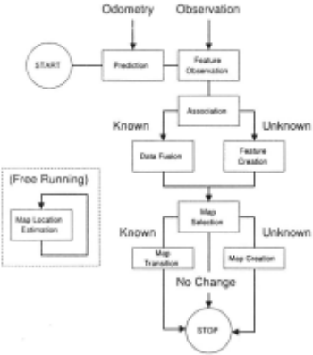
Figure 1 illustrates the processing steps that are performed by the algorithm. The four key elements are (1) SLAM pro cessing within local maps, (2) Map management (performing transitions between maps and creating new maps), (3) Map Location estimation (determining the best global location es timate for a submap), and (4) Computation of global state estimates for all features in a map. Each of these processes are described in detail below.
4.1 SLAM within local maps
At any one time, there is a single active map. For each map m, we compute a partial solution, p(xm(k)IZ~, A~, u:;,- 1 ), where Xm(k) designates the local map state, and Z~, A~, and u:;,- 1 represent subsets of the measurements, associ ations, and control inputs, respectively. Each measure ment is used in only a single map. (This is vital for ensuring consistency of the global Map Location estima tion process.) Each map m contains an estimated mean [x~(k)Tx!(k)T ... x~(k)TJT and covariance pm(k) cor responding to selected vehicle locations (for time steps when map m is the active map), and only a subset of the features. These estimates are the same as the location vectors [m,i]yj and associated uncertainty [m,i] :Ej for the features in the local map.
4.2 Map management
In our scheme, each map has a center, which is defined as the vehicle location at the time of the creation of a map. About this center is defined a region of radius r. This defines a bound of vehicle location and not feature locations - any feature that is observed from a position inside the map region will be added to the local map. The estimated location of the vehicle is used to deduce which map(s) the vehicle is in, and when to make transitions. When the vehicle travels more than r + h from the center, the vehicle is considered to have left the current map. The parameter h is a hysteresis term, to prevent excessive map switching. In the simulation results below, we use r = 15 and h = 5. (An alternative to circular map re gions is the use of convex hulls, but this makes no difference to the fundamental performance of the algorithm.)
We assume that the density of discernible features in a local area is bounded. This provides a bound on the number of features that can belong to a map.
When a vehicle leaves a map, we must determine which map (if any) the vehicle has transitioned to. A list of possible candidates is drawn up from a look up table indexed by quan tized vehicle locations. If more than one candidate exists, we choose the map with the lowest ID, i.e., the oldest map. If no candidates are found, then a new map is created at the cur rent location (a distance r + h from the center of the previous map). All of these operations can be performed in constant time.
4.3 Map Location estimation
Map Location estimation is the procedure by which global es timates for feature locations in each local map are improved, resulting in global convergence. This procedure is described as follows:
- Select a map p, to improve which is currently referenced to the root entity i.
- Create a set, N, containing the ID's of all nearby maps including p- the map to be improved.
- For each q E N , q =1- p create a set Cp,q of ID's of features that are present in both maps.
- For the frame :h attached to feature k E Cp,q· calculate its globally referenced location [q,-JTf and uncertainty [q,·J :Ef using the location estimate of feature k within map q and its current location estimate.
- Pick the map q* and entity ID k* such that:
- If q* = p and k* = i then stop. The map p cannot be improved
- Root Shift map p to k* from i-reference all entities in map p to a coordinate frame attached to entity k*.
- Replace Tf! and I:~ with (q' ·lTf. and [q' ,·l:Ef. respec tively.
For constant-time operation, Map Location estimation is performed only when the vehicle transitions from one map to another. Alternatively, the procedure can be performed peri odically (or at the end of the mission) to all maps. Multiple iterations result in global convergence to a near-optimal solu tion, but the computation complexity is no longer 0(1).
The work presented in this paper differs from that proposed in [Leonard and Feder, 2000] on the following counts:
- No vehicle information is carried between maps upon map transitions
- The SLAM scheme adopted within each map need not be based on a Kalman filter.
- Mapped entities are represented in local coordinate frames - one frame per map. In contrast, the DSM approach used multiple maps but all registered in one global coordinate frame.
4.4 Obtaining global location estimates for map features
Given an independent, consistent estimate of the location of a submap p (with root i) with respect to the global frame, G, we can produce a consistent global estimate of the location of any feature j in map p by composition of map and feature locations:
This estimate is consistent because T{! and (p,iJy 1 are inde pendent. (p, iJy 1 is "internal" to the map and T{! is "external" to the map.
The existence of a "shared" feature, s, between two maps p and q allows the location estimate T{!, of map p, (with root features), to be replaced with Tf!t. where
and w, the root of map q is any feature id in map q. Equation 7 should be interpreted as finding an alternative expression for the global location of a shared feature s using quantities associated with map q instead of p. As map p has a root at the shared feature s this expression is by definition an alternative expression for the map location. The minimization step of the algorithm is concerned with finding the best choice of shared features.
In the limit each map becomes internally fully correlated and the "min" operation will have no further effect so that for any feature j
where · is any choice of root. In other words no root-shifting and replace operation can be found that improves the global uncertainty of feature j. For the linear case
The maps are rooted on features and so as k --> oo then
and so
which is true for all choices of p and q. Therefore the glob ally referenced feature location uncertainty [·.-lr;J is the same independent of choice of map(·). The value ot this limiting value is clearly given by the smallest possible uncertainty in Map Location which is the uncertainty of the first feature ini tialized in the first map [Dissanayake et al., 2001]. This point is considered further in section 5.
5 Consistency and convergence
We begin by defining the term consistency with regard to an estimate x(kik) of an r.v x(k) at time k given all information up until time k. Defining the estimated error vector x(kik) £ x(k) -x(kik) and the estimate covariance as P(kik) we write the condition of consistency as:
To show that the global location estimates produced by Equa tion 6 are consistent, we rely on the following three proper ties: (1) local map state estimates (p,iJy 1 (obtained from the local SLAM solution [x~(k)Txr'(k)T ... :X~(kf]T) are consistent, (2) global state estimates for Map Locations r:r; are consistent, and (3) the composition of these two pieces of information - local state estimates within a map and global information concerning the location of the map - is consis tent.
The consistency of local maps follows directly from the properties of the Kalman filter which in the linear gaussian case is the optimal Bayesian estimator. Clearly, choosing to use a possibly inconsistent estimator such as the EKF in a nonlinear scenario will invalidate these claims. However, the LG case allows statements to be made regarding the underly ing properties of the CTS algorithm. In a non-linear imple mentation, the consistency of the LG case can be matched to an arbitrary degree by using Monte-Carlo estimators in each sub-map. Regardless of local estimation techniques, the CTS algorithm preserves its constant time property.
Local maps have three differences from the full solution (a) their base reference (root) is defined by one of the fea tures in the map, (b) relocation is periodically performed to re-initialize the local map when the vehicle transitions back into it, and (c) the base reference of the local map is peri odically shifted from one feature in the local map to another (Root Shifting). None of these three differences result in a Joss of consistency for the local SLAM solution.
The global Map Location estimate r;;; for a given map, m, is consistent because it is created via the composition of transformations derived from other local maps, and each local map is independent of other local maps. The composition of transformations from different local maps is a consistent operation (for the linear case).
Finally, the composition of the local map state estimates performed in Equation 6 is a consistent operation, because r;;; and [m,iJy 1 are independent of one another.
While the location estimates for different maps are corre lated with one another, and this correlation is not computed by the algorithm, the method in none-the-less consistent be cause this correlation is never needed. We never fuse Map Location estimates estimates, but rather, perform wholesale replacement. The algorithm keeps track of the best estimate for the global location of the root entity of a given map. A guiding principle of this algorithm is that estimated quantities that are "external" to a map never effect an internal quantity.
Due to the relocation step for map transitions, the infor mation from dead-reckoning measurements for the time step proceeding the map transition is effectively "lost". This in formation, however, does not affect absolute convergence but only the rate of convergence. Because relocation is a con sistent operation [Knight, 2002], each partial solution retains all the properties of a Kalman filter SLAM solution [Dis sanayake et al., 2001], and hence is provably consistent and convergent. Because each map is local with its base refer ence as one of the features in the map, in the limit the uncer tainty for each local map converges to zero [Dissanayake et al., 2001]. This implies that, in the limit, in any local map uti lizing only a subset of zk, the relationship between features becomes perfectly known as k --t oo. A consequence of this is that the covariance of the transformation between any two features, i and j, in any given map tends to zero as k --t oo. Hence, for local maps in which the base reference (root) is a feature in the local map, the covariance of any feature tends to zero. The key driver for convergence is the behavior in the first submap- submap 1. To illustrate this, consider a robot which moves swiftly outside submap 1 and spends the rest of its mission driving just outside submap 1 's borders. Eventu ally the maps bordering sub map 1 become completely known, including most of the features which appear in sub map 1. The global uncertainty of any feature in the bordering submaps can never be less than the global uncertainty in the location of submap 1. Hence, in this scenario, the root shifting mech anism can never decrease the global uncertainty of features in submap 1 (nothing has lower global uncertainty). However as soon as submap 1 is re-entered and begins to be refined, the global uncertainties of maps sharing features with map 1 can be reduced by root-shifting. Hence it is the precision of the first submap built (submap 1) that drives the ultimate performance of the entire system. In addition it is the preci sion of the first feature mapped within it that drives ultimate performance of submap 1.
Thus in the limit, the lower bound achieved in submap 1 is "inherited" by all other submaps. There are two differences between what occurs in submap I in comparison to a full co variance solution that couples estimates for all features in a single map: (a) submap 1 has fewer features in it, and (b) not all of the observations of features that are contained in submap 1 are processed in the submap 1 solution. We be lieve that consideration (a), the fact that submap 1 has fewer features in it, is what is sacrificed in this approach. Even if some measurements are ignored in submap 1 (vs. the full solution), in the limit as k ___, oo, both maps will converge to a well-defined lower bound. With enough additional time the submap 1 solution can "catch up" to the full solution. However, the fact that the full solution has more features enables in it cannot be compensated for, and hence the full solution achieves a slightly tighter bound. This in effect is the "cost" of computing multiple partial solutions and subse quently combining them, rather than computing one full solu tion. Our simulations have shown that this result is extremely small (as shown below in Figure 3).
6 Results
This section analyzes the behavior of the technique presented using simulations analysis. The simulations consider an
(x, y) "point" vehicle that moves in the plane with process noise Q of 0.05 or 0.01(Monte-Carlo) m/sec standard devia tion in both x and y and measurement noise R of 0.2 m/sec standard deviation in both x and y. Features are visible if they are within 23 meters of the vehicle location. One visible feature is selected at random each time step to generate the observations. Results are presented for three different scenar ios:
- a simulation involving six cycles through an environ ment in which eight maps are created (to illustrate basic error convergence behavior),
- Monte-Carlo analysis of 200 independent trials of a mis sion involving ten cycles through an environment in which twelve submaps are created (for empirical con sistency verification), and
- results off-line map adjustment for a mission involving a single cycle through an environment in which eighteen maps are created,
6.1 Comparison with the full covariance solution
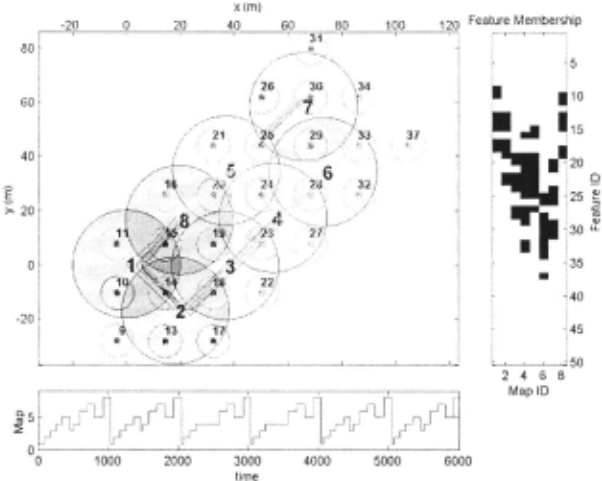
Figure 2 show the vehicle path for a mission in which eight maps are created. Figure 3 shows the vehicle error as a func tion of time as a function of time and active map ID. Spikes in the vehicle error estimate occur at each map transition when relocation (consistent re-initialization of the vehicle pose) is performed. This is particularly obvious towards the end of the experiment when the features are well known and subse quent observations swiftly bring the vehicle covariance down following relocation. Figure 4 shows the difference between the new method and the full solution in the determinant of er ror covariance for the feature marginals in each map, demon strating the tight convergence of the method to near-optimal estimates, while never going below the minimum permissible error bounds.
6.2 Monte-Carlo consistency testing
For the purposes of consistency testing, two relative states were logged in the active submap: (1) the difference between the first feature in the state vector and the vehicle, and (2) the difference between the first and second features in the state vector. These two states are stored in a single vector ym with covariance ym formed from the active map (with id m). This relative vector can be compared to the 'true' relative relationships declared by the simulator producing the noise corrupted measurements. The difference between these vec tors is the error vector y( k). They vector calculated for each map m will in general involve different features (by definition as each map contains a subset of the set of all features with only some features in common). However each estimated component of ym should be consistent, hence any sequence {ym 1 (1), ... , ymk (k)} ffi[O:k] E [1 : MJ where M is the total number of maps built, should also be consistent. Figure 6.2 illustrates the results obtained from Monte-Carlo exper iments of the CTS algorithm. The parameters used in the simulation of sensor data and its subsequent processing are given in Table 6.2. All the plots are concerned with the statis tical properties of y ( k). The first plot of Figure 6.2 shows the mean values of y( k) -the difference for each time step k be tween the "true" relative vector y and the the estimate y. The upper two plots correspond to the vehicle to feature relative states. Note how the error does not converge to a zero value owing to the continual injection of process noise (odometry errors etc) into the vehicle as it moves. The lower two plots however correspond to the error in the relative location of the first two features in what ever the active map is. No pro cess noise is added to the feature estimate covariances during the prediction stage of the estimation process. The result is the expected convergence to zero error. The second plot of Figure 6.2 shows the plots the characteristics of theN-run av erage of the NEES (Normalized Estimated Error Squared) of y(k). The 95% confidence region bounds for estimation con sistency are plotted on the same axes. the final plot of Figure 6.2 shows the normalized mean estimated error (NMEE) and the associated 95% confidence bounds of the hypothesis that the NMEE sequences are from a consistent estimator.
6.3 Off-line Adjustment
The root shifting operation which searches for a better repre sentation (in terms of uncertainty) of map location and fea tures need not be done as the vehicle transitions between maps. Table 6.3 shows the improvement in successively ap- T.me Step nmeStop plying the CTS algorithm to maps at the termination of the mission for a scenario with 18 maps. The simple approach adopted here begins with submap 2 and seeks to improve the map location estimate, it then progresses to submap 3 and so on until the highest index map has been adjusted. This then repeats until no maps show any further improvement. It is a topic of future research to determine, as a function of shared feature topography, the optimal adjustment sequence rather than the linear one used here. The adjustment was applied to a mission with a vehicle trajectory defined by six overlapping rectangles (similar to Figure 2 but the course was not repeated leading to a more uncertain collection of submaps at the end of the mission). The entries in the table are the percentage decrease in median disparity between the full covariance and CTS calculated feature uncertainties. As expected, the table shows no improvement for submap 1.
| Parameter | J Value |
|---|---|
| Monte-Carlo Runs Vehicle Process Noise (std) Sensor Noise (std) Cycle Length Cycles per run Total Distance Driven per run Loops per Cycle Initial Vehicle uncertainty Sensor Range Sensor Field of View Feature Density Map Radius Vehicle Velocity | 200 0.01 ms- 1 0.05 m 360 m 10 3600 m 2 0 m 25 m 100 deg Every 18m in x andy 15m 0.3 ms- 1 |
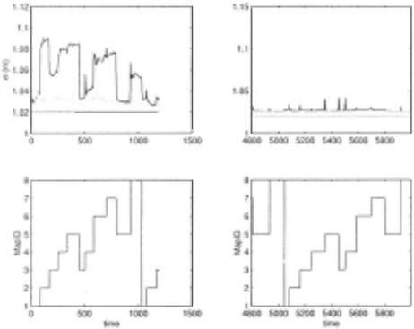
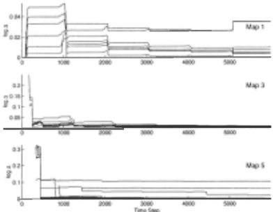
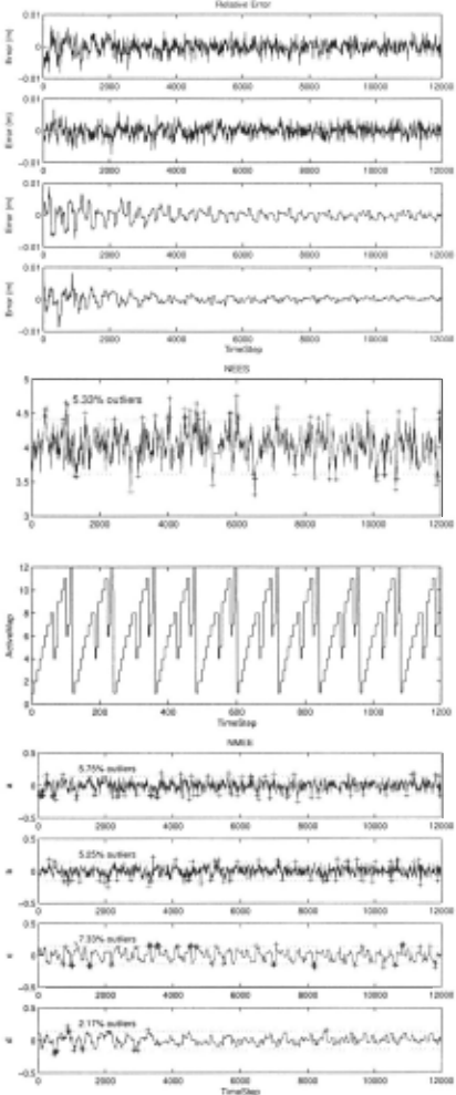
Figure 5: Monte-Carlo Consistency testing. The left hand plot shows the four components of the vector y which en codes the errors in relative positions of vehicle and the first two features <f'l, f2) in the state vector of the active map m (the map in which the vehicle is currently moving). The first upper two sequences are the x and y components of the error in the relative position between vehicle and f'l. The second two are the x andy components of the error in the relative po sitions of f'l and !2. The central plot is the NEES of y. The bounds are the 95% confidence intervals on the NEES vari able. The right hand plot shows the Normalized Mean Error (NMEE) for the components of y. For consistency the mean estimated error should be zero. The limits plotted are the 95% confidence interval bounds for the consistency hypothesis.
| I Map | I iteration I | I iteration 2 | iteration 3 |
|---|---|---|---|
| I 2 3 4 5 6 7 8 9 10 II 12 13 14 15 16 17 18 | 0.0 13.6 10.0 10.6 6.3 7. 1 20.7 1.8 6.6 3.5 1.6 15.0 3.7 4.1 4.5 7.5 14.4 12.9 | 0.0 13.6 16.8 18.9 13.0 12.6 25.4 7.1 8.3 5.0 6.3 17.8 5.4 5.5 6.0 9.0 22.1 12.9 | 0.0 13.6 16.8 18.9 17.9 12.6 26.6 8.5 13.5 9.5 7.6 19.0 10.1 9.6 10.2 13.4 22.1 12.9 |
7 Conclusion
In this paper, we have presented a new technique for SLAM with multiple maps that achieves consistency of global state estimates with with 0( I) time complexity. If the mobile robot is able to make repeated visits to all parts of the environ ment, by performing map improvement operations only when a map is exited, near-optimal convergence is demonstrated in constant-time.
In this approach, all SLAM filtering is performed in lo cal submaps. Each submap has an associated reference frame, whose global position is estimated using information from other submaps. The transition of the vehicle between submaps is consistently performed using relocation [Neira et al., 2002; Knight, 2002]. By never mixing information between maps, the method yields provably consistent global state estimates, while still achieving global convergence.
The method successfully exploits the fact that overlapping features are estimated in different maps. By changing the base reference of a map to be the feature within the map that has the "best" globally referenced position estimate, the global location estimates for all the features in a local region get improved via operations in other maps.
Ongoing research includes testing of the method with real data, the incorporation of probabilistic data association tech niques, and extension of the approach to the nonlinear case.
@inproceedings{ijcai2003p163,
  title     = {Consistent, Convergent, and Constant-Time SLAM},
  author    = {Leonard, John J. and Newman, Paul M.},
  booktitle = {Proceedings of the Eighteenth International Joint Conference on
               Artificial Intelligence, {IJCAI-03}},
  publisher = {International Joint Conferences on Artificial Intelligence},
  editor    = {Georg Gottlob and Toby Walsh},
  pages     = {1143--1149},
  year      = {2003},
  url       = {https://ijcai.org/proceedings/2003/163},
}
TY - CPAPER TI - Consistent, Convergent, and Constant-Time SLAM AU - Leonard, John J. AU - Newman, Paul M. T2 - Proceedings of the Eighteenth International Joint Conference on Artificial Intelligence, IJCAI-03 PB - International Joint Conferences on Artificial Intelligence PY - 2003 SP - 1143 EP - 1149 UR - https://ijcai.org/proceedings/2003/163 ER -Copied
Machine-readable versions of this paper, for tools and AI agents:





