Qualitative Simulation of Genetic Regulatory Networks: Method and Application

1 Introduction

It is now commonly accepted in biology that most interesting properties of an organism emerge from the interactions among its genes, proteins, metabolites, and other molecules. This implies that, in order to understand the functioning of an organism, the networks of interactions involved in gene regulation, metabolism, signal transduction, and other cellular and intercellular processes need to be elucidated.

A genetic regulatory network consists of a set of genes and their mutual regulatory interactions. The interactions arise from the fact that genes code for proteins that may control the expression of other genes, for instance by activating or inhibiting DNA transcription [Lewin, 1999]. The study of genetic regulatory networks has received a major impetus from the recent development of experimental techniques permitting the spatiotemporal expression levels of genes to be rapidly measured in a massively parallel way [Brown and Botstein, 1999]. However, in addition to experimental tools, computer tools for the modeling and simulation of gene regulation processes will be indispensable. As most genetic regulatory systems of interest involve many genes connected through interlocking positive and negative feedback loops, an intuitive understanding of their dynamics is hard to obtain.

Currently, only a few regulatory networks are wellunderstood on the molecular level, and quantitative information about the interactions is seldom available. This has stimulated an interest in modeling and simulation techniques developed within qualitative reasoning (QR) [Heidtke and Schulze-Kremer, 1998; Trelease et al., 1999]. A major problem with these approaches, based on well-known methods like QSIM [Kuipers, 1994] and QPT [Forbus, 1984], is their lack of upscalability. Following approaches in mathematical biology, de Jong and Page [2000] have proposed a qualitative simulation method capable of handling large and complex networks.

The aim of this paper is to generalize the latter method and to demonstrate its applicability to real networks of biological interest. The generalization of the method allows a broader range of regulatory interactions between genes to be expressed. This enables more complex systems to be analyzed, such as the network of interactions controlling the inititation of sporulation in the bacterium Bacillus subtilis. We have simulated the sporulation network using a model constructed from published reports of experiments. The simulations reveal that an additional interaction, proposed in the literature before but not yet experimentally identified, may be involved.

In the next section, we will discuss the class of equations being used to model genetic regulatory networks. The third section describes the qualitative simulation algorithm, focusing on the representation of the qualitative state of a regulatory system and the determination of state transitions by the simulation algorithm. The subsequent sections present the results of the analysis of the sporulation network as well as a discussion of the method in the context of related work.

2 Modeling genetic regulatory networks

2.1 Approximations of regulatory interactions

In order to model a genetic regulatory network, we first have to describe the regulatory interactions in an empirically valid and mathematically rigorous way. Consider a DNA-binding protein encoded by gene ✞ , activating the expression of a target gene ✟ . The rate of transcription of ✟ as a function of the concentration ✠ ✡ of the regulatory protein follows a sigmoid curve [Yagil and Yagil, 1971]. Below a threshold concentration ☞ ✡ ✌ ✎ the gene is hardly expressed at all, whereas above this threshold its expression rapidly saturates.

Sigmoid curves are also found in the case of more complex regulatory mechanisms. Consider the proteins J and K that forma dimer repressing the transcription of gene ✟ (Fig. 2(b)). Analysis of a kinetic model of this regulatory mechanism reveals that the rate of expression of ✟ depends in a sigmoidal fashion on the total concentrations ✠ ✡ and ✠ ✑ of J and K, respectively. That is, both J and K need to be available above their threshold concentrations for ✟ to be repressed.

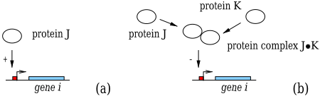
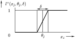
In the case of steep sigmoids, the combined effect of regulatory proteins on gene expression can be approximated by means of Boolean functions [Kauffman, 1993; Thomas and d'Ari, 1990]. Here we will rewrite a Boolean function in terms of step functions and arithmetic sums and multiplications, following the procedure of Plahte et al. [1998]. For the activator protein in Fig. 2(a), we thus obtain a regulation function ✜ ✢ ✠ ✡ ✥ ✧ ✩ ✫ ✭ ✢ ✠ ✡ ✰ ☞ ✡ ✥ , where ✫ ✭ ✢ ✥ is a step function (Fig. 5) and ✩ ✌ ✎ a rate parameter. Similarly, the effect of a regulatory protein repressing gene ✟ can be described by ✜ ✢ ✠ ✡ ✥ ✧ ✩ ✫ ✶ ✢ ✠ ✡ ✰ ☞ ✡ ✥ , with ✫ ✶ ✢ ✠ ✡ ✰ ☞ ✡ ✥ ✧ ✺ ✼ ✫ ✭ ✢ ✠ ✡ ✰ ☞ ✡ ✥ . The dimer repressor example in Fig. 2(b) leads to the function ✜ ❀ ✢ ✠ ✡ ✰ ✠ ✑ ✥ ✧ ✩ ❀ ✢ ✺ ✼ ✫ ✭ ✢ ✠ ✡ ✰ ☞ ✡ ✥ ✫ ✭ ✢ ✠ ✑ ✰ ☞ ✑ ✥ ✥ .

Although the above discussion has focused on the representation of interactions regulating the synthesis of proteins, it also applies to the degradation of proteins. Sigmoid relations are observed in the latter case as well, so that the logical approximations are valid. In order to formally distinguish protein degradation rates from protein synthesis rates, we will denote the former by ❇ ❀ instead of ✩ ❀ .

2.2 State equations

The dynamics of genetic regulatory networks can be modeled by a system of differential equations suggested by Mestl et al. [1995], extending earlier proposals by Glass and Kauffman [1973] and Thomas et al. [1990].

where ● is a vector of cellular protein concentrations. The state equations (1) define the rate of change of the concentration ✠ ❀ as the difference of the rate of synthesis ❊ ❀ ✢ ● ✥ and the rate of degradation ✼ ■ ❀ ✢ ● ✥ ✠ ❀ of the protein. Exogenous variables can be defined by setting ❈ ✠ ❀ ✧ ✎ .

The function ❊ ❀ ❯ ❱ ❳ ❨ ❩ ❬ ❱ ❨ ❪ is defined as

where ✜ ❀ ❛ ✢ ✥ is a regulation function and ❤ a possibly empty set of indices of regulation functions. The function ■ ❀ ✢ ✥ is defined analogously to (2), except that for reasons that will become clear below, we demand that ■ ❀ ✢ ● ✥ is strictly positive. Notice that for the above definitions of ❊ ❀ ✢ ✥ and ■ ❀ ✢ ✥ , the state equations (1) are piecewise-linear. Equations of this form, and their logical abstractions, have been well-studied in mathematical biology (e.g., [Lewis and Glass, 1991; Mestl et al., 1995; Thomas and d'Ari, 1990]).

Eqs. (1) and (2) generalize upon the formalism employed in [de Jong and Page, 2000] in two respects. First, the regulation functions ✜ ❀ ❛ ✢ ✥ may be the mathematical equivalent of any Boolean function, whereas in the earlier paper it was restricted to logical functions composed of Boolean products. Second, the regulation of protein degradation can now State equation for Spo0E:

State equation for AbrB:

Threshold inequalities:

Equilibrium inequalities: ❪ ❺ ♦ ♣ a113 ➁ ❸ ♣ a113 ❺ ④ ♣ a113 ⑧

Threshold inequalities:

Figure 3: State equations, threshold inequalities, and equilibrium inequalities for the genes (a) spo0E and (b) abrB in Fig. 1. The subscripts in the equations refer to the sporulation genes kinA ( ➈ ➉ ), spo0E ( ✫ ➊ ), spo0A ( ✫ ➉ ), sigA ( ➉ ), sigH ( ➋ ), and abrB (➉ ➌ ).

be modeled, whereas before the degradation rate was set to ■ ❀ ✢ ● ✥ ✧ ❇ ❀ . These extensions allow the structure of complex regulatory networks to be formalized in a convenient way.

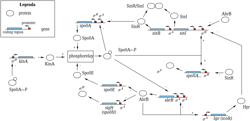
In Fig. 3 the state equations corresponding to two of the genes in the sporulation network of Fig. 1 are shown. The differential equation in (a) states that spo0E is transcribed at a rate ✩ ➍ ➎ from a ✙ ➏ -promoter when its repressor AbrB is below its threshold concentration ☞ ➑ ➒ ⑧ (i.e., ✫ ✶ ✢ ✠ ➑ ➒ ✰ ☞ ➑ ➒ ⑧ ✥ ✧ ✺ ). In addition, for transcription to commence, the sigma factor ✙ ➏ encoded by sigA needs to be available at a concentration above the threshold ☞ ➍ ➑ ⑧ (i.e., ✫ ✭ ✢ ✠ ➍ ➑ ✰ ☞ ➍ ➑ ⑧ ✥ ✧ ✺ ). Spo0E degrades at a rate proportional to its own concentration.

2.3 Threshold and equilibrium inequalities

In general, a protein encoded by a gene will be involved in different interactions at different threshold concentrations. Although exact numerical values will not usually be available, we can order the ➵ ❀ threshold concentrations of gene ✟ , which gives the threshold inequalities

The parameter ➼ ➽ ➚ ➪ denotes a maximum concentration for the protein denoted by ✟ .

For the sporulation gene abrB two thresholds are defined, ☞ ➑ ➒ ⑧ and ☞ ➑ ➒ ❻ . AbrB has two threshold concentrations: ☞ ➑ ➒ ⑧ and ☞ ➑ ➒ ❻ . The first threshold corresponds to the repression of spo0E, sigH, and other early sporulation genes by AbrB. The second threshold corresponds to the autoregulation of abrB during vegetative growth, when AbrB levels are at their highest. This motivates the ordering of the AbrB thresholds in Fig. 3(b): ☞ ➑ ➒ ⑧ ➲ ☞ ➑ ➒ ❻ .

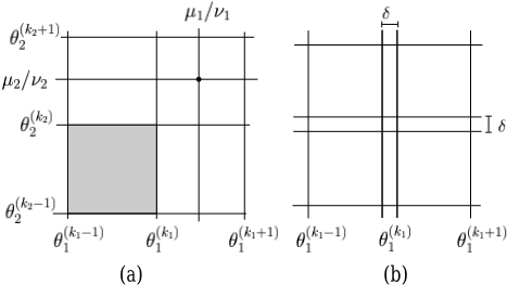
The a80 ✼ ✺ -dimensional threshold hyperplanes ✠ ❀ ✧ ☞ ➩ ✑ ➻ ➯ ❀ , ✺ ❖ ➈ ❀ ❖ ➵ ❀ divide the phase space box into regions, called regulatory domains (Fig. 4). Within each regulatory domain, the step function expressions in (2) can be evaluated, which reduces ❊ ❀ ✢ ✥ and ■ ❀ ✢ ✥ to sums of rate constants. That is, ❊ ❀ ✢ ✥ simplifies to some ➘ ❀ ➴ ➬ ❀ ✃ ❐ ❊ ❀ ✢ ● ✥ ❮ ❰ ❖ ● ❖ a207 a208 ● a209 , and ■ ❀ ✢ ✥ to some a210 ❀ ➴ a212 ❀ ✃ ❐ ■ ❀ ✢ ● ✥ ❮ ❰ ❖ ● ❖ a207 a208 ● a209 . The sets ➬ ❀ and a212 ❀ collect the different synthesis and degradation rates of the protein in different domains of the phase space.

It can be easily shown that all trajectories in a regulatory domain tend towards a single, stable steady state ● ✧ a215 a216 a218 , the target equilibrium, lying at the intersection of the hyperplanes ✠ ❀ ✧ ➘ ❀ a216 a210 ❀ [Glass and Kauffman, 1973; Mestl et al., 1995; Thomas and d'Ari, 1990]. The target equilibrium level ➘ ❀ a216 a210 ❀ of the protein concentration ✠ ❀ gives an indication of the strength of gene expression in the regulatory domain.

As in the case of threshold parameters, exact numerical values for the rate constants will not usually be available. However, it is possible order the possible target equilibrium levels of ✠ ❀ in different regions of the phase space with respect to the threshold concentrations. ➫ The resulting equilibrium inequalities define the strength of gene expression in a regulatory domain in a qualitative way, on the scale of ordered threshold concentrations. More precisely, for every ➘ ❀ ➴ ➬ ❀ , a210 ❀ ➴ a212 ❀ , we specify some a219 ❀ , ✺ ❖ a219 ❀ ➲ ➵ ❀ , such that

with special cases ✎ ➲ ➘ ❀ a216 a210 ❀ ➲ ☞ ➩ ➫ ➯ ❀ and ☞ ➩ ➺ ➻ ➯ ❀ ➲ ➘ ❀ a216 a210 ❀ ➲ ➼ ➽ ➚ ➪ .

Inspection of the state equations of AbrB shows that ➬ ➑ ➒ ✧ ❐ ✎ ✰ ✩ a221 a222 a209 and a212 ➑ ➒ ✧ ❐ ❇ a221 a222 a209 . The equilibrium level

a223 The equilibrium inequalities have also been called nullcline inequalities [de Jong and Page, 2000], because the equilibrium levels correspond to nullcline hyperplanes in the phase space.

✩ ➑ ➒ a216 ❇ ➑ ➒ is placed above the highest AbrB threshold, since otherwise a224 the concentration of AbrB would never be able to reach or maintain a level at which negative autoregulation takes place. This leads to the equilibrium inequalities ☞ ➑ ➒ ❻ ➲ ✩ ➑ ➒ a216 ❇ ➑ ➒ ➲ ➼ ➽ ➚ a221 a222 .

The threshold and equilibrium inequalities determine the sign of ❈ ✠ ❀ in a regulatory domain, and hence the local dynamics of the system. In fact, given a regulatory domain defined in dimension ✟ by ☞ ➩ ✑ ➻ ➯ ❀ ➲ ✠ ❀ ➲ ☞ ➩ ✑ ➻ ✭ ➫ ➯ ❀ , it can be shown that, if ➘ ❀ a216 a210 ❀ ➲ ☞ ➩ ✑ ➻ ➯ ❀ , then ❈ ✠ ❀ ➲ ✎ everywhere inside the regulatory domain. Similarly, if ➘ ❀ a216 a210 ❀ ✌ ☞ ➩ ✑ ➻ ✭ ➫ ➯ ❀ , then ❈ ✠ ❀ ✌ ✎ . On the other hand, if ☞ ➩ ✑ ➻ ➯ ❀ ➲ ➘ ❀ a216 a210 ❀ ➲ ☞ ➩ ✑ ➻ ✭ ➫ ➯ ❀ , then the sign of ❈ ✠ ❀ in the regulatory domain is not unique, written as ❈ ✠ ❀ a225 ✎ . In particular, ❈ ✠ ❀ ➲ ✎ on one side of the hyperplane ✠ ❀ ✧ ➘ ❀ a216 a210 ❀ , ❈ ✠ ❀ ✌ ✎ on the other side of the plane, and ❈ ✠ ❀ ✧ ✎ inside the plane.

2.4 Discontinuities in state equations

The question must be raised what happens on the threshold hyperplanes ✠ ❀ ✧ ☞ ➩ ✑ ➻ ➯ ❀ separating the regulatory domains, where the step functions, and hence the state equations, are not defined. Several solutions are possible for this non-trivial problem. In this paper we follow the approach of Plahte et al. [1994] and replace the discontinuous step functions by continuous ramp functions (Fig. 5). The solution of the PLDEs with step functions is then defined to be the solution of the DEs with ramp functions considered in the limit a228 ❬ ✎ .

a234

a235

a232

a233

a231

a238

a230

a231

a239

a230

a231

a237

a231

The use of ramp functions divides the phase space into regulatory domains separated by switching zones, regions in which one or more ✠ ❀ have a value in the a228 -interval a243 ☞ ➩ ✑ ➻ ➯ ❀ ✼ a228 a216 a244 ✰ ☞ ➩ ✑ ➻ ➯ ❀ a245 a228 a216 a244 a246 around a threshold ☞ ➩ ✑ ➻ ➯ ❀ . An example phase space with switching zones is shown in Fig. 4. Inside the regulatory domains, the DEs with ramp functions are equivalent to the PLDEs with step functions. Outside the regulatory domains, in the switching zones, the DEs with ramp functions may be nonlinear functions of the concentration variables. The switching zones separating the regulatory domains vanish and approach (intersections of) the threshold hyperplanes as a228 ❬ ✎ .

3 Qualitative simulation of genetic regulatory networks

The goal of qualitative simulation is to exploit the qualitative constraints on parameter values in order to predict the qualitative dynamics of a regulatory network. More specifically, we would like to know which regulatory domains can

a236

a237

be reached by some solution trajectory starting in the initial regulatory domain, for parameter values consistent with the specified threshold and equilbrium inequalities. A sequence of regulatory domains thus generated gives an indication of the evolution of the functional state of the system, as transitions between regulatory domains reflect changes in the synthesis and degradation rates of proteins.

3.1 Qualitative values, states, and behaviors

The analysis of PLDEs of the form (1) motivates the introduction of the qualitative value of a state variable and its derivative, as well as definitions of the qualitative state and qualitative behavior of the system. Let a248 ✢ a249 ✥ ✧ a248 ✢ ● ✰ ● ❩ ✰ a250 ✰ a251 ✰ a252 ✰ a249 ✥ be the solution of PLDEs with step functions describing a regulatory network on the time-interval a243 a249 ❩ ✰ a249 a253 a243 for given parameter values and initial conditions ● ✢ a249 ❩ ✥ ✧ ● ❩ .

Def. 1 (Qualitative value) Suppose that at some a249 ✌ a249 ❩ it holds that a248 ✢ a249 ✥ lies in a regulatory domain, such that ☞ ➩ ✑ ➻ ➯ ❀ ➲ a254 ❀ ✢ a249 ✥ ➲ ☞ ➩ ✑ ➻ ✭ ➫ ➯ ❀ for every ✟ ( ✺ ❖ ✟ ❖ a80 and ✺ ❖ ➈ ❀ ➲ ➵ ❀ ). The qualitative value a255 a0 ✢ a254 ❀ ✰ a249 ✥ of a254 ❀ ✢ a249 ✥ is given by the inequalities ☞ ➩ ✑ ➻ ➯ ❀ ➲ ✠ ❀ ➲ ☞ ➩ ✑ ➻ ✭ ➫ ➯ ❀ , while the qualitative value ❈ a255 a0 ✢ a254 ❀ ✰ a249 ✥ of ❈ a254 ❀ ✢ a249 ✥ is given by one of the inequalities ❈ ✠ ❀ ➲ ✎ , ❈ ✠ ❀ ✌ ✎ , ❈ ✠ ❀ a225 ✎ , depending on the sign of ❈ a254 ❀ ✢ a249 ✥ in the regulatory domain.

The definition can be straightforwardly generalized to the case of regulatory domains bounded by ✠ ❀ ✧ ✎ or ✠ ❀ ✧ ➼ ➽ ➚ ➪ . Notice that the qualitative value is not defined in the switching zones around the threshold hyperplanes.

Def. 2 (Qualitative state) The qualitative state a255 ✫ ✢ a248 ✰ a249 ✥ for a248 at a249 is given by the vectors a255 a0 ✢ a248 ✰ a249 ✥ and ❈ a255 a0 ✢ a248 ✰ a249 ✥ of qualitative values.

A qualitative state associated with a regulatory domain can be interpreted as representing a functional state of the regulatory system. Each protein concentration has a value lying between two consecutive thresholds, and is either tending towards one of the threshold values, or evolving towards a value between the thresholds.

Def. 3 (Qualitative behavior) The qualitative

behavior a255 ➌ ✢ a248 ✥ of a248 is given by the sequence of qualitative states a255 ✫ ✢ a248 ✰ a249 ✥ on a243 a249 ❩ ✰ a249 a253 a243 .

A qualitative behavior defines a succession of qualitative states of the regulatory system. It is not difficult to show that every solution a248 of (1) can be abstracted into a unique qualitative behavior.

3.2 Qualitative simulation algorithm

In terms of the above definitions, the qualitative simulation procedure can be formulated as follows [Kuipers, 1994]. Given initial qualitative values ✂ ✄ ❩ , describing the initial protein concentrations ● , the simulation algorithm computes the initial qualitative state a255 ✫ ❩ , and then determines all possible transitions from a255 ✫ ❩ to successor qualitative states. The generation of successor states is repeated in a recursive manner until all qualitative states reachable from the initial qualitative state have been found.

The possible transitions from a qualitative state are determined by the rule below.

Figure 6: Continuity constraints for the qualitative values a255 a0 ❀ ✰ ❈ a255 a0 ❀ and a255 a0 ✗ ❀ ✰ ❈ a255 a0 ✗ ❀ of two qualitative states a255 ✫ and a255 ✫ ✗ defined on adjacent regulatory domains. Valid for ✺ ➲ ➈ ❀ ➲ ➵ ❀ ✼ ✺ , the constraints can be easily generalized to the case of qualitative values ✎ ❖ ✠ ❀ ➲ ☞ ➩ ➫ ➯ ❀ and ☞ ➩ ➺ ➻ ➯ ❀ ➲ ✠ ❀ ❖ ➼ ➽ ➚ ➪ .

Def. 4 (State transition) Let a255 ✫ and a255 ✫ ✗ be two qualitative states associated with adjacent regulatory domains. A transition from a255 ✫ to a255 ✫ ✗ is possible, if for every ✟ , ✺ ❖ ✟ ❖ a80 , such that a255 a0 ❀ ✙ ✧ a255 a0 ✗ ❀ , the qualitative values a255 a0 ❀ ✰ ❈ a255 a0 ❀ and a255 a0 ✗ ❀ ✰ ❈ a255 a0 ✗ ❀ satisfy the continuity constraints in Fig. 6.

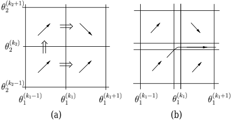
Fig. 7(a) illustrates the application of the rule. Intuitively formulated, the rule says that a transition from one qualitative state to another is possible, if a trajectory may cross the switching zone separating the regulatory domains of the qualitative states.

A simulation algorithm based on Def. 4 is described in [de Jong and Page, 2000]. The qualitative states and transitions generated by the algorithm form a state transition graph. The graph may contain cycles and states without successors, which are together referred to as attractors. Since the number of possible qualitative states is finite, every path in the state transition graph will reach an attractor at some point. Each path running from the initial qualitative state a255 ✫ ❩ to an attractor forms a possible qualitative behavior of the regulatory system.

3.3 Properties of simulation algorithm

Given a model and initial qualitative values ✂ ✄ ❩ , what can be said about the correctness of the behaviors produced by qualitative simulation? We define a set ✢ of possible solutions of (1) on a243 a249 ❩ ✰ a249 a253 a243 , such that for every a248 ➴ ✢ the numerical values of a250 , a251 , and a252 satisfy (3)-(4), and a255 a0 ✢ a248 ✰ a249 ❩ ✥ ✧ ✂ ✄ ❩ .

The ultimate aim of qualitative simulation is to determine the set ✣ ✤ of qualitative behaviors, such that (1) for every a248 ➴ ✢ there is a ➌ ➴ ✣ ✤ , such that a255 ➌ ✢ a248 ✥ ✧ ➌ (soundness), and (2) for every ➌ ➴ ✣ ✤ there is a a248 ➴ ✢ , such that a255 ➌ ✢ a248 ✥ ✧ ➌ (completeness).

Unfortunately, the simulation algorithm based on Def. 4 is not sound. A trajectory may enter a switching zone from a regulatory domain, and then escape through other switching zones to enter another, possibly non-adjacent regulatory domain (Fig. 7(b)). As a consequence, the simulation algorithm may overlook qualitative state transitions. We found that the practical consequences of such omissions are limited, since qualitative states not directly reachable by a transition are often indirectly reachable by a sequence of transitions.

Completeness of the simulation algorithm has neither been proven nor disproven, but seems difficult to guarantee given the behavioral complexity that can be attained by models of the form (1) [Lewis and Glass, 1991].

3.4 Genetic Network Analyzer

The simulation method has been implemented in Java 1.2, in a program calledGNA (Genetic Network Analyzer). ➳ The program reads and parses input files specifying the model of the system (state equations, threshold and equilibrium inequalities) and the initial state. From this information it produces a state transition graph. Extensions of the simulation algorithm allow all qualitative states and their transitions to be generated, as well as the completion and simulation of models with unspecified threshold and equilibrium inequalities.

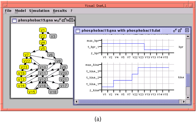
GNA is accessible through a graphical user-interface, which allows the network of interactions between genes to be displayed, as well as the state transition graph resulting from the simulation. In addition, the user can analyze the attractors with their basins of attraction, and focus on qualitative behaviors to study the temporal evolution of protein concentrations in more detail (Fig. 8).

4 Application: sporulation in B. subtilis

The method and its implementation have been used to study the regulatory network underlying the initiation of the sporulation process in the Gram-positive soil bacterium Bacillus subtilis [Grossman, 1995; Hoch, 1993]. Under conditions of nutrient deprivation, B. subtilis can decide not to divide and form a dormant, environmentally-resistant spore instead. The decision to either divide or sporulate is made by a complex regulatory network integrating various environmental, cellcyle, and metabolic signals.

A schematic representation of the core of this network, displaying key genes and their regulatory interactions, is shown in Fig. 1. The central component of the network is a phosphorylation pathway, a phosphorelay, which transfers phosphates from the KinA kinase to the Spo0A regulator. Above a certain threshold, the phosphorylated formof Spo0A (Spo0A✦ P) activates various genes that commit the bacterium to sporulation. An example is the spoIIA operon, which encodes the transcription factor ✙ ✧ , essential for the development of the forespore. The flux of phosphate across the phosphorelay,

✔ GNA is available from the authors upon request.

(b)

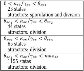
Figure 8: (a) GNA output for the equilibrium inequalities ✎ ➲ ✩ ➍ ➎ a216 ❇ ➍ ➎ ➲ ☞ ➍ ➎ ⑧ . The left window shows the state transition graph with a qualitative behavior running from the initial qualitative state V1 to the attractor state V15. In the right window the temporal evolution of the qualitative value of Hpr and KinA for this behavior can be followed. (b) Summary of simulation results for an initial state expected to induce sporulation, while varying the equilibrium inequalities for Spo0E. The simulations take between 0.5 and 3 seconds to complete on a Sun Ultra 10 workstation.

and hence the concentration of Spo0A ✦ P, is controlled by various external signals influencing the activity of pathway components. In addition, the flux of phosphate is regulated by Spo0A ✦ P itself, through a number of direct and indirect feedback loops involving abrB, sinI, sinR, and other genes.

Using the extensive literature on B. subtilis sporulation, and the Subtilist database at the Institut Pasteur, we have formulated state equations and appropriate parameter inequalities for every gene in the network. In total, the mathematical model consists of 10 state equations, 10 threshold inequalities, and 30 equilibrium inequalities. In the rare cases that the literature did not unambiguously determine the parameter inequalities, we have systematically explored the alternatives and selected those that permit the observed behavior of the bacterium to be reproduced.

The behavior of B. subtilis has been simulated from a variety of initial states, reflecting different physiological conditions. For example, fig. 8(a) shows the simulation results for an initial state reflecting a perturbation of the vegetative growth conditions, when the protein kinase KinA autophosphorylates in response to an external signal indicating a state of nutritional deprivation. Under these conditions, a state transition graph with two attractors is produced, corresponding to states in which the bacterium continues to divide (V3) or initiates spore formation (V15 and V18). Both states may be reached, depending on the exact values of the parameters satisfying the threshold and equilibrium inequalities.

In order to obtain result consistent with experimental data, we found that the target equilibrium concentrations of Spo0E have to be placed below the lowest threshold concentrations ( ✎ ➲ ✩ ➍ ➎ a216 ❇ ➍ ➎ ➲ ☞ ➍ ➎ ⑧ ). That is, we need to assume that spo0E expression levels are quite weak. When other equilibrium inequalities are chosen, the simulations predict that sporulation cannot be initiated under appropriate conditions, contrary to what is observed (Fig. 8(b)). In fact, Spo0Emediates the negative autoregulation of Spo0A ✦ P, and thus prevents a critical concentration of Spo0A ✦ P to accumulate.

The above choice of parameter constraints is troublesome, because it implies that Spo0E cannot exert any influence on the decision to sporulate, since its concentration will not reach the threshold levels above which it can block the phosphate flux through the phosphorelay. The simulation results thus suggest that the network in Fig. 1, based on interactions reported in the literature, may be incomplete. As a remedy, we could postulate that an unknown signal decreases the activity of Spo0E at the onset of sporulation. Molecular studies of the interaction of Spo0E with components of the phosporelay suggest the existence of such a cellular factor which remains as of yet unidentified [Ohlsen et al., 1994].

5 Discussion

We have presented an implemented method for the qualitative simulation of genetic regulatory systems that can handle large and complex networks of genes and interactions. The method is a generalization of the method in [de Jong and Page, 2000], in that it allows a larger class of regulatory relationships between genes to be modeled. In the first place, there are no restrictions on the logical functions that can be represented by (2). This permits complex regulatory interactions to be included in the models, as illustrated by the state equation for abrB in Fig. 3(b). In the second place, the regulation of protein degradation can be taken into account. Although this feature of the method has not been used in the sporulation example, it turned out to be crucial in modeling the network controlling the induction of the lytic cycle following phage ➘ infection of E. coli (results not shown here).

The applicability of the method to actual regulatory networks has been demonstrated by an analysis of the large and complex network underlying the initiation of sporulation in B. subtilis. The analysis has resulted in a suggestion to complete the model compiled from the sporulation literature, which shows the potential of the method as a tool to focus further exprimentation. To our knowledge, qualitative simulation of genetic regulatory networks of the size and complexity considered in this paper has not been undertaken thus far.

Upscaling of the simulation method is achieved by modeling genetic regulatory systems by a class of piecewise-linear differential equations imposing strong constraints on the local dynamics of the system. Besides in molecular genetics, PLDEs of this form have been used in other biological domains, for instance in population biology. In order to effectively apply the constraints, the representation of the qualitative state of the system and the simulation algorithm are adapted to the mathematical structure of the equations.

Adaptation to a specific class of models is the principal respect in which the method presented in this paper differs from well-known QR methods like QPT and QSIM [Forbus, 1984; Kuipers, 1994]. A major difference with QSIM is that the qualitative state of a regulatory system is described on a higher level of abstraction. In particular, the behavior inside a regulatory domain is abstracted into a single qualitative state, making use of the fact that inside a regulatory domain either ❈ ✠ ❀ ➲ ✎ , ❈ ✠ ❀ ✌ ✎ , or ❈ ✠ ❀ a225 ✎ . In QSIM one would have to distinguish an exponentially growing number of qualitative states inside and on the boundary of a regulatory domain.

Approximating step functions by infinitely steep ramp functions allows a precise definition of the behavior of the system in the threshold planes, and hence of the possible successors of a qualitative state. The state transition rule in Def. 4 is simple and intuitively clear, but does not preserve soundness of the algorithm. Even though the practical limitations of this may be limited, the development of state transition rules guaranteeing soundness is an important topic for further research.

The B. subtilis example suggest an approach to validate hypothesized models of genetic regulatory networks. Given temporal gene expression patterns observed under certain physiological conditions in wild-type or mutant strains of the bacterium, one can develop algorithms to systematically search the space of freely adjustable parameter inequalities to find constraints for which the model is able to account for the observations. Extensions of this type would allow the simulation method presented in this paper to evolve into a more general modeling tool.

Acknowledgments The authors would like to thank I. Vatcheva and three anonymous referees for comments on a previous version of this paper.