An On-line Decision-Theoretic Golog Interpreter

1 Introduction

The aim of this paper is to provide a new on-line architecture of designing controllers for autonomous agents. Specifically, we explore controllers for mobile robots programmed in DTGolog, an extension of the high-level programming language Golog. DTGolog aims to provide a seamless integration of a decision-theoretic planner based on Markov decision processes with an expressive set of program control structures available in Golog. The motivation for this research is provided in [Boutilier et al., 2000], and we ask the reader to consult that paper for additional technical details and arguments why neither model-based planning, nor programming alone can manage the conceptual complexity of devising controllers for mobile robots. The DTGolog interpreter described in [Boutilier et al., 2000] is an off-line interpreter that computes the optimal conditional policy a0 , the probability ✁ ✂ that a0 can be executed successfully and the expected utility ☎ of the policy. The semantics of a DTGolog program ✁ is defined by the predicate ✆ ✝ ✟ ✡ ☞ ✍ ✏ ✁ ✓ ✟ ✓ ✖ ✓ a0 ✓ ☎ ✓ ✁ ✂ ✙ , where ✟ is a starting situation and ✖ is a given finite horizon. The policy a0 returned by the off-line interpreter is a Golog program consisting of the sequential composition of agent actions, senseEffect ✏ ✛ ✙ sensing actions (which serve to identify a real outcome of a stochastic action ✛ ) and conditionals (if ✜ then a0 ✢ else a0 ✤ ), where ✜ is a situation calculus formula that provides a test condition to decide which branch of a policy the agent should take given the result of sensing. The interpreter looks ahead up to the last choice point in each branch of the program (say, between alternative primitive actions), makes the choice and then proceeds backwards recursively, deciding at each choice point what branch is optimal. It is assumed that once the off-line DTGolog interpreter has computed an optimal policy, the policy is given to the robotics software to control a real mobile robot.

However this off-line architecture has a number of limitations. Imagine that we are interested in executing a program (✁ ✢ ✥ ✁ ✤ ) where both sub-programs ✁ ✢ and ✁ ✤ are very large nondeterministic DTGolog programs designed to solve 'independent' decision-theoretic problems: ✁ ✤ is supposed to start in a certain set of states, but from the perspective of ✁ ✤ it is not important what policy will be used to reach one of those states. Intuitively, in this case we are interested in computing first an optimal policy a0 ✢ (that corresponds to ✁ ✢ ), executing a0 ✢ in the real world and then computing and executing an optimal policy a0 ✤ . But the off-line interpreter can return only the optimal policy a0 that corresponds to the whole program ( ✁ ✢ ✥ ✁ ✤ ), spending on this computation more time than necessary: to compute and execute a0 ✤ it is not relevant what decisions have to bemade during the execution of a0 ✢ . The second limitation becomes evident if in addition to senseEffect sensing actions serving to identify outcomes of stochastic actions, we need to explicitly include sensing actions in the program (and those sensing actions cannot be characterized as stochastic actions with a fixed finite set of outcomes). Imagine that we are given a program

✁ ✢ ✥ ✏ a0 ✦ ✓ ✡ ✙ ★ ✪ ✏ ✬ ✍ ✭ ✏ ✡ ✙ ✙ ✱ ✥ ✟ ✝ ✬ ✟ ✝ ✏ ✴ ✓ ✦ ✓ ✡ ✙ ✥ if ✜ then ✁ ✤ else ✁ ✵ ✷ , where ✟ ✝ ✬ ✟ ✝ ✏ ✴ ✓ ✦ ✓ ✡ ✙ is a sensing action that returns at time ✡ a measurement ✦ of a quantity ✴ (e.g., the current coordinates, the battery voltage) and the condition ✜ depends on the real data ✦ that will be returned by sensors (in the program above ✁ ✢ ✓ ✁ ✤ ✓ ✁ ✵ are sub-programs, the choice operator a0 binds variables ✦ and ✡ and the test ✬ ✍ ✭ ✏ ✡ ✙ ✱ grounds the current time). Intuitively, we want to compute an optimal policy a0 ✢ (corresponding to ✁ ✢ ) off-line, execute a0 ✢ in the real world, sense ✦ and then compute and execute an optimal policy a0 ✤ that corresponds to the conditional Golog program in brackets. But the off-line interpreter is not able to compute an optimal policy if a given program includes explicit sensing actions and no information is available about the possible results of sensing. Note that the nondeterministic choice operator a0 (it occurs in front of the program) should not be confused with policies a0 ✢ and a0 ✤ computed by an interpreter.

We propose to compute and execute optimal policies online using a new incremental decision theoretic interpreter. It works in a step-by-step mode. Given a Golog program ✁ and a starting situation ✟ , it computes an optimal policy a0 and the program ✁ ✻ that remains when a first action ✛ in a0 will be executed. At the next stage, the action ✛ is executed in the real world. The interpreter gets sensory information to identify which outcome of ✛ has actually occurred if ✛ is a stochastic action: this may require doing a sequence of sensing actions on-line. The action ✛ (and possibly sensing actions performed after that) results in a new situation. Then the cycle of computing an optimal policy and remaining program, executing the first action and getting sensory information (if necessary) repeats until the program terminates or execution fails. In the context of the incremental on-line execution, we define a new programming operator ✍ ✁ ✡ ✽ ✾ ✽ ❀ ✝ ✏ ✁ ✙ that limits the scope of search performedby the interpreter. If ✁ is thewhole program, then no computational efforts are saved when the interpreter computes an optimal policy from ✁ , but if the programmer writes ✍ ✁ ✡ ✽ ✾ ✽ ❀ ✝ ✏ ✁ ✢ ✙ ✥ ✁ ✤ , then the on-line incremental interpreter will compute and execute step-by-step the Golog program ✁ ✢ without looking ahead to decisions that need to be made in ✁ ✤ . If the programmer knows that the sensing action ✟ ✝ ✬ ✟ ✝ ✏ ✴ ✓ ✦ ✓ ✡ ✙ is necessary to evaluate the condition ✜ , then using the program

the required information about ✴ will be obtained before the incremental interpreter will proceed to the execution of the conditional. If the sensing action ✟ ✝ ✬ ✟ ✝ ✏ ✴ ✓ ✦ ✓ ✡ ✙ hasmany different outcomes, then this approach gives computational advantages over the off-line approach to computing an optimal policy.

Thus, the incremental interpretation of the decisiontheoretic Golog programs needs an account of sensing (formulated in the situation calculus) that will satisfy several criteria which naturally arise in the robotics context. There are several accounts of sensing in the situation calculus that address different aspects of reasoning about sensory and physical actions [Bacchus et al., 1995; De Giacomo and Levesque, 1999a; 1999b; Funge, 1998; Grosskreutz, 2000; Lakemeyer, 1999; Levesque, 1996; Pirri and Finzi, 1999; Scherl and Levesque, 1993].

Below we propose a new representation of sensing that simplifies reasoning about results of sensing, does not require consistency of sensory information with the domain theory, leads to a natural and sound implementation and has connections with representation of knowledge and sensing considered in [Reiter, 2000].

In Section 2 we recall the representation of the decision theoretic domain introduced in [Boutilier et al., 2000]. InSection 3 we propose a representation for sensing actions and consider several examples. In section 4 we consider the on-line incremental decision-theoretic interpreter. Section 5 discusses connections with previously published papers.

2 The decision theoretic problem representation

The paper [Boutilier et al., 2000] introduces the representation of problem domains that do not include sensing actions. The representation is based on the distinction between agent actions (which can be either deterministic or stochastic) and nature's actions which correspond to separate outcomes of a stochastic agent action. Nature's actions are considered deterministic. They cannot be executed by the agent itself, therefore they never occur in policies which the agent executes. When the agent does a stochastic action ✛ in a situation ✟ , nature chooses one of the outcomes ✬ of that action and the situation ❂ ✍ ✏ ✬ ✓ ✟ ✙ is considered as one of resulting situations. In accordance with this perspective, the evolution of a stochastic transition system is specified by precondition and successor state axioms which never mention stochastic agent actions, but mention only deterministic agent actions and nature's actions. In [Boutilier et al., 2000], it is suggested to characterize the DTGolog problem domain by: 1) the predicate ✛ ❄ ✝ ✬ ✡ ❇ ❈ ✡ ✽ ✍ ✬ ✏ ✛ ✙ which holds if ✛ is an agent action, 2) the predicate ✟ ✡ ✍ ❈ ✖ ✛ ✟ ✡ ✽ ❈ ✏ ✛ ✓ ✟ ✓ ✬ ✙ meaning that nature's action ✬ is one of outcomes of the stochastic agent action ✛ in the situation ✟ , 3) the function symbol ✁ ✂ ✍ ❋ ✏ ✬ ✓ ✟ ✙ that denotes the probability of nature's action ✬ in situation ✟ , and 4) the predicate senseCond ✏ ✬ ✓ ✜ ✙ specifying the test condition ✜ serving to identify the outcome ✬ of the last stochastic action, 5) the function symbol ✂ ✝ ✭ ✛ ✂ ❂ ✏ ❂ ✍ ✏ ✛ ✓ ✟ ✙ ✙ denotes rewards and costs as functions of the current situation ❂ ✍ ✏ ✛ ✓ ✟ ✙ , the action ✛ or both.

As an example, imagine a robot moving between different locations: the process of going is initiated by a deterministic action ✟ ✡ ✛ ✂ ✡ ■ ✍ ✏ ❏ ✢ ✓ ❏ ✤ ✓ ✡ ✙ but is terminated by a stochastic action ✝ ✬ ❂ ■ ✍ ✏ ❏ ✢ ✓ ❏ ✤ ✓ ✡ ✙ that may have two different outcomes: successful arrival ✝ ✬ ❂ ■ ✍ ▲ ✏ ❏ ✢ ✓ ❏ ✤ ✓ ✡ ✙ and unsuccessful stop in a place different from the destination ✝ ✬ ❂ ■ ✍ ❖ ✏ ❏ ✢ ✓ ❏ ✵ ✓ ✡ ✙ (the robot gets stuck in the hall or cannot enter an office because its door is closed). We represent the process of moving between locations ❏ ✢ and ❏ ✤ by the relational fluent ❄ ✍ ✽ ✬ ❄ ✏ ❏ ✢ ✓ ❏ ✤ ✓ ✟ ✙ and represent a (symbolic) location of the robot by the relational fluent ✂ ✍ ❋ ✍ ✡ a80 ✍ ❈ ✏ ❏ ✓ ✟ ✙ meaning that ❏ (the office of an employee, the hall or the main office) is the place where the robot is. The transitions in the stochastic dynamical system describing the robot's motion are characterized by the following precondition and successor state axioms.

Poss ❘ startGo ❘ ❙ ❚ ❯ ❙ ❱ ❯ ❲ ❳ ❯ ❨ ❳ ❩ ❬ ❘ ❫ ❙ ❯ ❙ ❴ ❳ going ❘ ❙ ❯ ❙ ❴ ❯ ❨ ❳ ❛ robotLoc ❘ ❙ ❚ ❯ ❨ ❳ ❯

Poss ❘ endGoS ❘ ❙ ❚ ❯ ❙ ❱ ❯ ❲ ❳ ❯ ❨ ❳ ❩ going ❘ ❙ ❚ ❯ ❙ ❱ ❯ ❨ ❳ ❯ Poss ❘ endGoF❘ ❙ ❚ ❯ ❙ ❱ ❯ ❲ ❳ ❯ ❨ ❳ ❩ ❫ ❙ ❴ ❜ going❘ ❙ ❚ ❯ ❙ ❴ ❯ ❨ ❳ ❛ ❙ ❴ ❞ ❢ ❙ ❱ ❯ going ❘ ❙ ❯ ❙ ❴ ❯ ❤ ✐ ❘ ❥ ❯ ❨ ❳ ❳ ❩ ❘ ❫ ❲ ❳ ❥ ❢ startGo ❘ ❙ ❯ ❙ ❴ ❯ ❲ ❳ ❧ going❘ ❙ ❯ ❙ ❴ ❯ ❨ ❳ ❛ ❬ ❘ ❫ ❲ ❳ ❥ ❢ endGoS❘ ❙ ❯ ❙ ❴ ❯ ❲ ❳ ❧ going ❘ ❙ ❯ ❙ ❴ ❯ ❨ ❳ ❛ ❬ ❘ ❫ ❲ ❯ ❙ ❴ ❴ ❳ ❥ ❢ endGoF ❘ ❙ ❯ ❙ ❴ ❴ ❯ ❲ ❳ ❜

The real outcome ✬ of a stochastic agent action ✛ can be identified only from sensory information. This information has to be obtained by executing sensing actions. In the following section we propose a new representation for sensing actions providing a seamless integration with the representation considered in this section.

3 Sensing actions

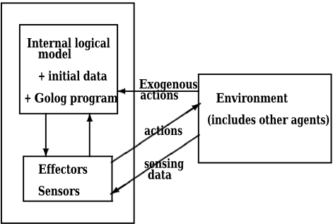
In contrast to physical actions, sensing actions do not change any properties of the external world, but return values measured by sensors. Despite this difference, it is convenient to treat both physical and sensing actions equally in successor state axioms. This approach is justifiable if fluents represent what the robot 'knows' about the world (see Figure 1). More specifically, let the high-level control module of the robot be provided with the internal logical model of the world (the set of precondition and successor state axioms) and the axiomatization of the initial situation. The programmer expresses ♣ in this axiomatization his (incomplete) knowledge of the initial situation and captures certain important effects of the robot's actions, but some other effects and actions of other agents may remain unmodeled. When the robot does an action in the real world (i.e., the high-level control module sends a command to effectors and effectors execute this command), it does not know directly and immediately what effects in reality this action will produce: the high-level control module may only compute expected effects using the internal logical model. Similarly, if the robot is informed about actions executed by external agents, the high-level control module may compute expected effects of those exogenous actions (if axioms account for them). Thus, from the point of view of the programmer who designed the axioms, the high-level control module maintains the set of beliefs that the robot has about the real world. This set of beliefs needs feedback from the real world because of possible contingencies, incompleteness of the initial information and unobserved or unmodeled actions executed by other agents. To gain the feedback, the high-level control module requests information from sensors and they return required data. We find it convenient to represent information gathered from sensors by an argument of the sensing action: a value of the argument will be instantiated at the run time when the sensing action will be executed. Then, all the high-level control module needs to know is the current situation (action log): expected effects of actions on fluents can be computed from the given sequence of physical and sensing actions.

In the sequel, we consider only deterministic sensing actions, but noisy sensing actions can be represented as well.

We suggest representing sensing actions by the functional symbol ✟ ✝ ✬ ✟ ✝ ✏ ✇ ✓ ✦ ✓ ✡ ✙ where ✇ is what to sense, ✦ is term representing a run time value returned by the sensors and ✡ is time; the predicate ✟ ✝ ✬ ✟ ✝ ❇ ❈ ✡ ✽ ✍ ✬ ✏ ✛ ✙ is true whenever ✛ is a sensing action. We proceed to consider several examples of successor state axioms that employ our representation.

1. Let ✟ ✝ ✬ ✟ ✝ ✏ ② ✍ ✍ ✂ ❂ ✓ ❏ ✓ ✡ ✙ be the sensing action that returns the pair ❏ ③ ✏ ④ ✓ ⑤ ✙ of geometric coordinates of the current robot location on the two-dimensional grid and ❄ ✂ ✽ ❂ a80 ✍ ❈ ✏ ④ ✓ ⑤ ✓ ✟ ✙ be a relational fluent that is true if ✏ ④ ✓ ⑤ ✙ are the coordinates of the robot's location in ✟ . In this example we assume that all actions are deterministic (we do this only to simplify the exposition of this example). The process of moving (represented by the relational fluent

⑥ ✐ ⑦ ⑨ ⑩ ❶ ❘ ❷ ❚ ❯ ❸ ❚ ❯ ❷ ❱ ❯ ❸ ❱ ❯ ❨ ❳ ) from the grid location ✏ ④ ✢ ✓ ⑤ ✢ ✙ to the point ✏ ④ ✤ ✓ ⑤ ✤ ✙ is initiated by the deterministic instantaneous action ❨ ❲ ❥ ❹ ❲ ❺ ✐ ⑦ ❼ ❘ ❷ ❚ ❯ ❸ ❚ ❯ ❷ ❱ ❯ ❸ ❱ ❯ ❲ ❳ and is terminated by the deterministic action ❼ ⑩ ❤ ❺ ✐ ⑦ ❼ ❘ ❷ ❚ ❯ ❸ ❚ ❯ ❷ ❱ ❯ ❸ ❱ ❯ ❲ ❳ . The robot may also change its location if it is transported by an external agent from one place to another: the exogenous actions ✡ ✛ ❽ ✝ ✏ ④ ✢ ✓ ⑤ ✢ ✓ ✡ ✙ and ✁ ☎ ✡ ✏ ④ ✤ ✓ ⑤ ✤ ✓ ✡ ✙ account for this (and the fluent ✡ ✂ ✛ ✬ ✟ ✁ ✍ ✂ ✡ ✝ ❂ ✏ ✟ ✙ represents the process of moving the robot by an external agent). The following successor state and precondition axioms characterize aforementioned fluents and actions.

❄ ✂ ✽ ❂ a80 ✍ ❈ ✏ ④ ✓ ⑤ ✓ ❂ ✍ ✏ ✛ ✓ ✟ ✙ ✙ ❾ ✏ ✏ ❿ ✡ ✓ ❏ ✙ ✛ ③ ✟ ✝ ✬ ✟ ✝ ✏ ② ✍ ✍ ✂ ❂ ✓ ❏ ✓ ✡ ✙ ➁ ④ ② ✂ ❂ ✏ ❏ ✙ ③ ④ ➁ ⑤ ② ✂ ❂ ✏ ❏ ✙ ③ ⑤ ✙ ➃ ✏ ➄ ✡ ✂ ✛ ✬ ✟ ✁ ✍ ✂ ✡ ✝ ❂ ✏ ✟ ✙ ➁ ✏ ❿ ✡ ✓ ④ ✻ ✓ ⑤ ✻ ✙ ✛ ③ endMove✏ ④ ✻ ✓ ⑤ ✻ ✓ ④ ✓ ⑤ ✓ ✡ ✙ ✙ ➃ ✏ ✡ ✂ ✛ ✬ ✟ ✁ ✍ ✂ ✡ ✝ ❂ ✏ ✟ ✙ ➁ ✏ ❿ ✡ ✙ ✛ ③ ✁ ☎ ✡ ✏ ④ ✓ ⑤ ✓ ✡ ✙ ✙ ➃ ❄ ✂ ✽ ❂ a80 ✍ ❈ ✏ ④ ✓ ⑤ ✓ ✟ ✙ ➁ ➄ ✏ ❿ ✡ ✓ ④ ✻ ✓ ⑤ ✻ ✙ ✛ ③ ✁ ☎ ✡ ✏ ④ ✻ ✓ ⑤ ✻ ✓ ✡ ✙ ➁ ➄ ✏ ❿ ❏ ✓ ✡ ✙ ✛ ③ ✟ ✝ ✬ ✟ ✝ ✏ ② ✍ ✍ ✂ ❂ ✓ ❏ ✓ ✡ ✙ ➁ ➄ ✏ ❿ ④ ✓ ⑤ ✓ ④ ✻ ✓ ⑤ ✻ ✓ ✡ ✙ ✛ ③ endMove ✏ ④ ✓ ⑤ ✓ ④ ✻ ✓ ⑤ ✻ ✓ ✡ ✙ ✓

where ④ ② ✂ ❂ ✏ ❏ ✙ ✓ ⑤ ② ✂ ❂ ✏ ❏ ✙ denote, respectively, ④ and ⑤ components of the current robot location ❏ .

❲

✾ ✍ ✦ ✽ ✬ ❄ ✏ ④ ✢ ✓ ⑤ ✢ ✓ ④ ✤ ✓ ⑤ ✤ ✓ ❂ ✍ ✏ ✛ ✓ ✟ ✙ ✙ ❾ ✏ ❿ ✡ ✙ ✛ ③ startMove ✏ ④ ✢ ✓ ⑤ ✢ ✓ ④ ✤ ✓ ⑤ ✤ ✓ ✡ ✙ ➃ ✾ ✍ ✦ ✽ ✬ ❄ ✏ ④ ✢ ✓ ⑤ ✢ ✓ ④ ✤ ✓ ⑤ ✤ ✓ ✟ ✙ ➁ ➄ ✏ ❿ ✡ ✙ ✛ ③ endMove ✏ ④ ✢ ✓ ⑤ ✢ ✓ ④ ✤ ✓ ⑤ ✤ ✓ ✡ ✙ ★ ❹ ❥ ⑩ ❨ ➊ ✐ ❹ ❲ ❼ ❤ ❘ ❤ ✐ ❘ ❥ ❯ ❨ ❳ ❳ ❩ ❘ ❫ ❲ ❯ ❷ ❯ ❸ ❳ ❥ ❢ ❲ ❥ ➌ ❼ ❘ ❷ ❯ ❸ ❯ ❲ ❳ ❧ ❲ ❹ ❥ ⑩ ❨ ➊ ✐ ❹ ❲ ❼ ❤ ❘ ❨ ❳ ❛ ❬ ❘ ❫ ❲ ❯ ❷ ❴ ❯ ❸ ❴ ❳ ❥ ❢ ➊ ➍ ❲ ❘ ❷ ❴ ❯ ❸ ❴ ❯ ❲ ❳ ❧ ❘ ❬ ❫ ❷ ❯ ❸ ❯ ❷ ❴ ❯ ❸ ❴ ❳ ⑥ ✐ ⑦ ⑨ ⑩ ❶ ❘ ❷ ❯ ❸ ❯ ❷ ❴ ❯ ❸ ❴ ❳ ❛ ❶ ❹ ⑨ ❤ ➎ ✐ ➏ ❘ ❷ ❯ ❸ ❯ ❨ ❳ ❛ ❘ ❫ ❲ ❯ ❙ ❳ ❥ ❢ ❨ ❼ ⑩ ❨ ❼ ❘ ➐ ✐ ✐ ❹ ❤ ❯ ❙ ❯ ❲ ❳ ❛ ❘ ❷ ➐ ❹ ❤ ❘ ❙ ❳ ❞ ❢ ❷ ❧ ❸ ➐ ❹ ❤ ❘ ❙ ❳ ❞ ❢ ❸ ❳ ❜ Poss ❘ startMove❘ ❷ ❚ ❯ ❸ ❚ ❯ ❷ ❱ ❯ ❸ ❱ ❯ ❲ ❳ ❯ ❨ ❳ ❩ ❬ ❲ ❹ ❥ ⑩ ❨ ➊ ✐ ❹ ❲ ❼ ❤ ❘ ❨ ❳ ❛ ❬ ❘ ❫ ❷ ❯ ❸ ❯ ❷ ❴ ❯ ❸ ❴ ❳ ⑥ ✐ ⑦ ⑨ ⑩ ❶ ❘ ❷ ❯ ❸ ❯ ❷ ❴ ❯ ❸ ❴ ❯ ❨ ❳ ❛ ❶ ❹ ⑨ ❤ ➎ ✐ ➏ ❘ ❷ ❚ ❯ ❸ ❚ ❯ ❨ ❳ ❯ Poss ❘ endMove❘ ❷ ❚ ❯ ❸ ❚ ❯ ❷ ❱ ❯ ❸ ❱ ❯ ❲ ❳ ❯ ❨ ❳ ❩ ⑥ ✐ ⑦ ⑨ ⑩ ❶ ❘ ❷ ❚ ❯ ❸ ❚ ❯ ❷ ❱ ❯ ❸ ❱ ❯ ❨ ❳ ❯ Poss❘ ❲ ❥ ➌ ❼ ❘ ❷ ❯ ❸ ❯ ❲ ❳ ❯ ❨ ❳ ❩ ❬ ❲ ❹ ❥ ⑩ ❨ ➊ ✐ ❹ ❲ ❼ ❤ ❘ ❨ ❳ ❛ ❶ ❹ ⑨ ❤ ➎ ✐ ➏ ❘ ❷ ❯ ❸ ❯ ❨ ❳ ❛ ❬ ❘ ❫ ❷ ❚ ❯ ❸ ❚ ❯ ❷ ❱ ❯ ❸ ❱ ❳ ⑥ ✐ ⑦ ⑨ ⑩ ❶ ❘ ❷ ❚ ❯ ❸ ❚ ❯ ❷ ❱ ❯ ❸ ❱ ❯ ❨ ❳ ❯ Poss❘ ➊ ➍ ❲ ❘ ❷ ❯ ❸ ❯ ❲ ❳ ❯ ❨ ❳ ❩ ❲ ❹ ❥ ⑩ ❨ ➊ ✐ ❹ ❲ ❼ ❤ ❘ ❨ ❳ ❜

Imagine that in the initial situation the robot stays at (0,0); later, at time 1, it starts moving from (0,0) to (2,3), but when the robot stops at time 11 and senses its coordinates at time 12, its sensors tell it that it is located at (4,4). The sensory information is inconsistent with the expected location of the robot, but this discrepancy can be attributed to unobserved actions of an external agent who transported the robot. Hence, the final situation is not

➓ ➔ ❢ ❤ ✐ ❘ ❨ ❼ ⑩ ❨ ❼ ❘ ➐ ✐ ✐ ❹ ❤ ❯ ❘ → ❯ → ❳ ❯ ➣ ↔ ❳ ❯ ❤ ✐ ❘ endMove❘ ↕ ❯ ↕ ❯ ↔ ❯ ➙ ❯ ➣ ➣ ❳ ❯ ❤ ✐ ❘ startMove❘ ↕ ❯ ↕ ❯ ↔ ❯ ➙ ❯ ➣ ❳ ❯ ➓ ➛ ❳ ❳ ❳ ❯

as we originally expected, but the situation resulting from the execution of exogenous actions ✡ ✛ ❽ ✝ ✏ ➜ ✓ ➝ ✓ ➞ ✢ ✙ and ✁ ☎ ✡ ✏ ➟ ✓ ➟ ✓ ➞ ✤ ✙ , in the situation when the robot ends moving, followed by the sensing action. The exogenous actions occurred at unknown times ➞ ✢ ✓ ➞ ✤ (we may say about the actual history only that ➠ ➠ ➡ ➞ ✢ ➤ ➞ ✤ ➡ ➠ ➜ ). 1

1. The robot can determine its location using data from sonar and laser sensors. But if the last action was not sensing coordinates ✏ ④ ✓ ⑤ ✙ , then the current locationcanbedetermined

1 In the sequel, we do not consider how the discrepancy between results of a deterministic action and observations obtained from sensors can be explained by occurrences of unobserved exogenous actions. However, our example indicates that inconsistency between physical and sensory actions can be resolved by solving a corresponding diagnostic problem (e.g., see [McIlraith, 1998]).

from the previous location and the actions that the robot has executed. ➦ The process of going from ❏ to ❏ ✻ is initiated by the deterministic action ✟ ✡ ✛ ✂ ✡ ■ ✍ ✏ ❏ ✓ ❏ ✻ ✓ ✡ ✙ and is terminated by the stochastic action ✝ ✬ ❂ ■ ✍ ✏ ❏ ✓ ❏ ✻ ✓ ✡ ✙ (axiomatized in Section 2).

✂ ✍ ❋ ✍ ✡ a80 ✍ ❈ ✏ ❏ ✓ ❂ ✍ ✏ ✛ ✓ ✟ ✙ ✙ ❾ ✏ ❿ ✡ ✓ ✦ ✓ ④ ✓ ⑤ ✙ ✛ ③ ✟ ✝ ✬ ✟ ✝ ✏ ② ✍ ✍ ✂ ❂ ✓ ✦ ✓ ✡ ✙ ➁ ④ ② ✂ ❂ ✏ ✦ ✙ ③ ④ ➁ ⑤ ② ✂ ❂ ✏ ✦ ✙ ③ ⑤ ➁ ✏ ✏ ❿ ✁ ✙ ❏ ③ office ✏ ✁ ✙ ➁ inOffice✏ ❏ ✓ ④ ✓ ⑤ ✙ ➃ ❏ ③ ➩ ✛ ❏ ❏ ➁ ➄ ✏ ❿ ✁ ✙ inOffice✏ office ✏ ✁ ✙ ✓ ④ ✓ ⑤ ✙ ✙ ➃ ✏ ❿ ✡ ✓ ❏ ✢ ✙ ✛ ③ ✝ ✬ ❂ ■ ✍ ▲ ✏ ❏ ✢ ✓ ❏ ✓ ✡ ✙ ➃ ✏ ❿ ✡ ✓ ❏ ✢ ✙ ✛ ③ ✝ ✬ ❂ ■ ✍ ❖ ✏ ❏ ✢ ✓ ❏ ✓ ✡ ✙ ➃ ✂ ✍ ❋ ✍ ✡ a80 ✍ ❈ ✏ ❏ ✓ ✟ ✙ ➁ ➄ ✏ ❿ ✡ ✓ ❏ ✤ ✓ ❏ ✵ ✓ ✦ ✙ ✏ ✛ ③ ✟ ✝ ✬ ✟ ✝ ✏ ② ✍ ✍ ✂ ❂ ✓ ✦ ✓ ✡ ✙ ➁ ✛ ③ ✝ ✬ ❂ ■ ✍ ▲ ✏ ❏ ✤ ✓ ❏ ✵ ✓ ✡ ✙ ➁ ✛ ③ ✝ ✬ ❂ ■ ✍ ❖ ✏ ❏ ✤ ✓ ❏ ✵ ✓ ✡ ✙ ✙ ★

where the predicate inOffice ✏ ❏ ✓ ④ ✓ ⑤ ✙ is true if the pair ✏ ④ ✓ ⑤ ✙ is inside of the office ❏ , the functional symbols bottomY✏ ❏ ✙ , topY ✏ ❏ ✙ , rightX ✏ ❏ ✙ and leftX ✏ ❏ ✙ represent coordinates of top left and bottom right corners of a rectangle that contains the office ❏ inside: When the robot stops and senses coordinates, it determines its real location and the high-level control module can identify the outcome of the stochastic action ✝ ✬ ❂ ■ ✍ ✏ ❏ ✓ ❏ ✻ ✓ ✡ ✙ : whether the robot stopped successfullyor failed to arrive at the intended destination.

3. Let ❄ ✽ ✦ ✝ ✏ ✽ ✡ ✝ ✾ ✓ ✁ ✝ ✂ ✟ ✍ ✬ ✓ ✡ ✙ be a stochastic action that has two different outcomes: ❄ ✽ ✦ ✝ ▲ ✏ ✽ ✡ ✝ ✾ ✓ ✁ ✝ ✂ ✟ ✍ ✬ ✓ ✡ ✙ - the robot gives successfully an ✽ ✡ ✝ ✾ to ✁ ✝ ✂ ✟ ✍ ✬ at time ✡ - and ❄ ✽ ✦ ✝ ❖ ✏ ✽ ✡ ✝ ✾ ✓ ✁ ✝ ✂ ✟ ✍ ✬ ✓ ✡ ✙ - the action of giving an ✽ ✡ ✝ ✾ to ✁ ✝ ✂ ✟ ✍ ✬ is unsuccessful. Let ✟ ✝ ✬ ✟ ✝ ✏ ❇ ❈ ❽ ✬ ✓ ✦ ✓ ✡ ✙ be the action of sensing whether delivery of the ✽ ✡ ✝ ✾ to ✁ ✝ ✂ ✟ ✍ ✬ was successful or not: if it was, then delivery is acknowledged and ✦ =1, if not - the result of sensing is ✦ =0. The following successor state axiom characterizes how the fluent hasCoffee✏ ✁ ✝ ✂ ✟ ✍ ✬ ✓ ✟ ✙ changes from situation to situation: whenever the robot is in the office of ✁ ✝ ✂ ✟ ✍ ✬ and it senses that one of its buttons was pressed, it is assumed that the ✁ ✝ ✂ ✟ ✍ ✬ pressed a button to acknowledge that she has a coffee. From this sensory information, the high-level control module can identify whether the outcome of ❄ ✽ ✦ ✝ ✏ ✽ ✡ ✝ ✾ ✓ ✁ ✝ ✂ ✟ ✍ ✬ ✓ ✡ ✙ was successful or not.

It is surprisingly straightforward to use regression in our setting to solve the forward projection task. Let ➵ be a background axiomatization of the domain (a set of successor state axioms, precondition axioms, unique name axioms and a set of first order sentences whose only situation term is ▲ ➸ ) and let ✜ ✏ ✟ ✙ be a situation calculus formula that has the free variable ✟ as the only situational argument. Supposewe are given a ground situational term ▲ that may mention both physical and sensing actions. The forward projection task is to determine whether

Regression is a computationally efficient way of solving the forward projection task [Reiter, 2000; Pirri and Reiter, 1999] when ▲ does not mention any sensing actions. The representation introduced above allows us to use regression also in the case when ▲ mentions sensing actions explicitly. Thus, we can use regression to evaluate tests ✏ ✜ ✙ ✱ in Golog programs with sensing actions: no modifications are required. In addition, our approach allows us to use an implementation in Prolog considered in [Reiter, 2000]. There is also an interesting connection between our representation of 'beliefs' and sensing and the approach to knowledge-based programming [Reiter, 2000]. In [Soutchanski, 2001] we show that his approach and our approach to the solution of the forward projection task (with sensing actions) are equivalent.

4 The incremental on-line DTGolog interpreter

The incremental DTGolog interpreter uses the predicate IncrBestDo✏ ✁ ✢ ✓ ✟ ✓ ✁ ✤ ✓ ✖ ✓ a0 ✓ ☎ ✓ ✁ ✂ ✙ and the predicate ❖ ✽ ✬ ✛ ❏ ✏ ✁ ✓ ✟ ✓ a0 ✓ ☎ ✙ . The former predicate takes as input the Golog program ✁ ✢ , starting situation ✟ , horizon ✖ and returns the optimal conditional policy a0 , its expected utility ☎ , the probability of success ✁ ✂ , and the program ✁ ✤ that remains after executing the first action from the policy a0 . The latter predicate tells when the execution of the policy completes: ❖ ✽ ✬ ✛ ❏ ✏ ✁ ✓ ✟ ✓ a0 ✓ ☎ ✙ is true if either the program ✁ is ➼ ✽ ❏ (the null program) or ▲ ✡ ✍ ✁ (a zero cost action that takes the agent to an absorbing state meaning that the execution failed), or if the policy a0 is ➼ ✽ ❏ or ▲ ✡ ✍ ✁ . In all these cases, ☎ is simply the reward associated with the situation ✟ . Note that in comparison to BestDo, IncrBestDo has an additional argument ✁ ✤ representing the program that remains to be executed.

IncrBestDo ✏ ✁ ✢ ✓ ✟ ✓ ✁ ✤ ✓ ✖ ✓ a0 ✓ ☎ ✓ ✁ ✂ ✙ is defined inductively on the structure of a Golog program ✁ ✢ . Below we consider its definition in the case when the program ✁ ✢ begins with a deterministic agent action.

If a deterministic agent action ✛ is possible in situation ✟ , then we compute the optimal policy a0 ✻ of the remaining program ✁ ✢ , its expected utility ☎ ✻ and the probability of successful termination ✁ ✂ ✻ . Because ✛ is a deterministic action, the probability ✁ ✂ ✻ that the policy a0 ✻ will complete successfully is the same as for the program itself; the expected utility ☎ is a sum of a reward for being in ✟ and the expected utility of continuation ☎ ✻ . If ✛ is not possible, then the remaining program is ➼ ✽ ❏ , and the policy is the Stop action, the expected utility is the reward in ✟ and the probability of success is 0.

Other cases are defined similarly to ✆ ✝ ✟ ✡ ☞ ✍ , e.g., if the programbegins with the finite nondeterministic choice ✏ a0 ✏ ④ ✃ ❐ ✙ ✁ ✙ ✥ ✁ ✻ , where ❐ is the finite set ❒ ❈ ✢ ✓ ★ ★ ★ ✓ ❈ ❮ ❰ and the choice binds all free occurrences of ④ in ✁ to one of the elements:

where ✁ ➺ a208 a209 means substitution of ❈ for all free occurrences of ④ in ✁ . Thus, the optimal policy ✁ ✍ ❏ corresponds to the element ❈ in ❐ that delivers the best execution. Note that the remaining program ✁ a207 is the same on the both sides of the definition.

Recall that policies are Golog programs as well. Moreover, if ✁ is a Golog program that contains many nondeterministic choices, the optimal policy a0 computed from ✁ is a conditional program that does not involve any nondeterministic choices. This observation suggests that programmers may wish to take advantage of the structure in a decision theoretic problem and use explicit search control operators that limit bounds where the search for an optimal policy has to concentrate. In addition to the standard set of Golog programming constructs, we introduce two new operators: ❏ ✍ ❈ ✛ ❏ ✏ ✁ ✙ and ✍ ✁ ✡ ✽ ✾ ✽ ❀ ✝ ✏ ✁ ✙ . Intuitively a210 , the program ❏ ✍ ❈ ✛ ❏ ✏ ✁ ✢ ✙ ✥ ✁ ✤ means the following. First, compute the optimal policy a0 ✢ corresponding to the subprogram ✁ ✢ , then compute the optimal policy a0 corresponding to the program a0 ✢ ✥ ✁ ✤ . If both sub-programs ✁ ✢ and ✁ ✤ are highly nondeterministic, then using the operator ❏ ✍ ❈ ✛ ❏ ✏ ✁ ✢ ✙ the programmer indicates where the computational efforts can be saved: there is no need in looking ahead further than ✁ ✢ to compute a0 ✢ . Thus, in the case that a Golog program begins with ❏ ✍ ❈ ✛ ❏ ✏ ✁ ✙

IncrBestDo✏ ❏ ✍ ❈ ✛ ❏ ✏ ✁ ✢ ✙ ✥ ✁ ✤ ✓ ✟ ✓ ✁ a207 ✓ ✖ ✓ a0 ✓ ☎ ✓ ✁ ✂ ✙ ➽ ➾ ➚ ③ ✏ ❿ ✁ ✓ a0 ✢ ✓ ☎ ✢ ✓ ✁ ✂ ✢ ✙ IncrBestDo ✏ ✁ ✢ ✥ ➼ ✽ ❏ ✓ ✟ ✓ ✁ ✓ ✖ ✓ a0 ✢ ✓ ☎ ✢ ✓ ✁ ✂ ✢ ✙ ➁ IncrBestDo ✏ a0 ✢ ✥ ✁ ✤ ✓ ✟ ✓ ✁ a207 ✓ ✖ ✓ a0 ✓ ☎ ✓ ✁ ✂ ✙ ★

The construct ❏ ✍ ❈ ✛ ❏ ✏ ✁ ✢ ✙ limits the search, but once the policy a0 ✢ was computed and the first action in a0 ✢ was executed, the remaining part of the program has no indication where the search may concentrate. For this reason, the programmer may find convenient to use another search control operator that once used persists in the remaining part of the program until the program inside the scopes of that operator terminates. This operator is called ✍ ✁ ✡ ✽ ✾ ✽ ❀ ✝ ✏ ✁ ✙ and is specifiedby the following abbreviation.

IncrBestDo✏ ✍ ✁ ✡ ✽ ✾ ✽ ❀ ✝ ✏ ✁ ✢ ✙ ✥ ✁ ✤ ✓ ✟ ✓ ✁ a207 ✓ ✖ ✓ a0 ✓ ☎ ✓ ✁ ✂ ✙ ➽ ➾ ➚ ③ ✏ ❿ ✁ ✻ ✙ IncrBestDo ✏ ✁ ✢ ✥ ➼ ✽ ❏ ✓ ✟ ✓ ✁ ✻ ✓ ✖ ✓ a0 ✓ ☎ ✓ ✁ ✂ ✙ ➁ ✏ ✁ ✻ a211 ③ ➼ ✽ ❏ ➁ ✁ a207 ③ ✏ ✍ ✁ ✡ ✽ ✾ ✽ ❀ ✝ ✏ ✁ ✻ ✙ ✥ ✁ ✤ ✙ ➃ ✁ ✻ ③ ➼ ✽ ❏ ➁ ✁ a207 ③ ✁ ✤ ✙ ★

According to this specification, an optimal policy a0 can be computed without looking ahead to the program ✁ ✤ ; hence, using ✍ ✁ ✡ ✽ ✾ ✽ ❀ ✝ ✏ ✁ ✢ ✙ a programmer can express a domain specific procedural knowledge to save computational efforts. Note that when ✁ ✻ is Nil, i.e. there will be nothing in ✁ ✢ to execute after doing the only action in a0 , the remaining program ✁ a207 contains only ✁ ✤ .

4.1 Implementing the on-line interpreter

Given the definitions of IncrBestDo mentioned in the previous sub-section, we can consider now the on-line interpretation coupled with execution of Golog programs. The definitions of IncrBestDo ✏ ✁ ✢ ✓ ✟ ✓ ✁ ✤ ✓ ✖ ✓ a0 ✓ ☎ ✓ ✁ ✂ ✙ translate directly into Prolog clauses (we omit them here). The on-line interpreter calls the off-line incrBestDo(E,S,ER,H,Pol1,U1,Prob1) interpreter to compute an optimal policy from the given program expression a213 , gets the first action of the optimal policy, commits to it, does it in the physical world, then repeats with the rest of the program. The following is such an interpreter implemented in Prolog:

online(E,S,H,Pol,U) :- incrBestDo(E,S,ER,H,Pol1,U1,Prob1), ( final(ER,S,H,Pol1,U1), Pol=Pol1, U=U1 ; reward(R,S), Pol1 = (A : Rest), ( agentAction(A), not stochastic(A,S,L), doReally(A), /*execute A in reality*/ !, /* commit to the result */ online(ER,do(A,S),H,PolFut,UFut), Pol=(A : PolFut), U is R + UFut ; senseAction(A), doReally(A), /* do sensing */ !, /*commit to results of sensing*/ online(ER,do(A,S),H,PolFut,UFut), Pol=(A : PolFut), U is R + UFut ; agentAction(A), stochastic(A,S,L), doReally(A), /*execute A in reality*/ !, /* commit to the result */

senseEffect(A,S,SEff), diagnose(SEff,L,SN), /*What happened?*/ online(ER,SN,H,PolFut,UFut), Pol=(A : PolF), U is R + UFut ) ).

The on-line interpreter uses the Prolog cut (!) to prevent backtracking to the predicate ❂ ✍ a214 ✝ ✛ ❏ ❏ ⑤ : we need this because once actions have been actually performed in the physical world, the robot cannot undo them.

In addition to predicates mentioned in section 2, the on-line interpreter uses the predicate senseEffect ✏ ❇ ✓ ▲ ➠ ✓ ▲ ➜ ✙ , the predicate diffSequence ✏ ❇ ✓ ▲ ✝ ✇ ✙ and the predicate ❂ ✽ ✛ ❄ ✬ ✍ ✟ ✝ ✏ ▲ ➜ ✓ a215 ☎ ✡ ❈ ✍ ✾ ✝ ✟ a80 ✽ ✟ ✡ ✓ ▲ ➝ ✙ . We describe below their meaning and show their implementation in Prolog.

Given the stochastic action ❇ and the situation ▲ ➠ , the predicate senseEffect ✏ ❇ ✓ ▲ ➠ ✓ ▲ ➜ ✙ holds if ▲ ➜ is the situation that results from doing a number of sensing actions necessary to differentiate between outcomes of the stochastic action ❇ . The predicate diffSequence ✏ ❇ ✓ ▲ ✝ ✇ ✙ holds if ▲ ✝ ✇ is the sequence of sensing actions (✛ ✢ ✥ ✛ ✤ ✥ ★ ★ ★ ✥ ✛ ❮ ) specified by the programmer in the domain problem representation: this sequence is differentiating if after doing all actions in the sequence the action chosen by 'nature' as the outcome of stochastic action ❇ can be uniquely identified.

senseEffect(A,S,SE) :- diffSequence(A,Seq), getSensorInput(S,Seq,SE). getSensorInput(S,A,do(A,S)) :- senseAction(A), doReally(A). /*connect to sensors, get data for a free variable in A */ getSensorInput(S1,(A : Rest),SE) :- doReally(A), /* connect to sensors, get data */ getSensorInput(do(A,S1),Rest,SE).

The predicate ❂ ✽ ✛ ❄ ✬ ✍ ✟ ✝ ✏ ▲ ➠ ✓ a80 ✓ ▲ ➜ ✙ takes as its first argument the situation resulting from getting a sensory input: it contains 'enough' information to disambiguate between different possible outcomes of the last stochastic action ❇ . The second argument is the list a80 of all outcomes that nature may choose if the agent executes the stochastic action ❇ in ▲ ➠ and the third argument is the situation that is the result of nature's action which actually occurred. We can identify which action nature has chosen using the set of mutually exclusive test conditions senseCond ✏ ✬ a216 ✓ ✜ a216 ✙ , where ✜ a216 is a term representing a situation calculus formula: if ✜ a216 holds in the current situation, then we know that nature has chosen the action ✬ a216 ( ✬ a216 belongs to the list a80 ).

diagnose(SE,[N],do(N,SE)) :- senseCond(N,C), holds(C,SE). diagnose(SE,[N|Outcomes],SN):- senseCond(N,C), ( holds(C,SE), SN=do(N,SE) ; not holds(C,SE), diagnose(SE,Outcomes,SN) ).

Successful tests of the implementation described here were conducted in a real office environment on a mobile robot B21 manufactured by RWI. The low-level software was initially developed in the University of Bonn to control Rhino, another B21 robot, see [Burgard et al., 1999] for details. The tests of implementation demonstrated that using the expressive set of Golog operators it is straightforward to encode domain knowledge as constraints on the given large MDP problem. The operator ✍ ✁ ✡ ✽ ✾ ✽ ❀ ✝ ✏ ✁ ✙ proved to be useful in providing heuristics which allowed to compute sub-policies in real time. These preliminary a210 tests have brought several new important issues, e.g., how the computation of a new policy off-line can proceed in parallel with executing actions from the policy on-line.

5 Discussion

The incremental Golog interpreter based on the singlestep ➞ ✂ ✛ ✬ ✟ -semantics is introduced in [De Giacomo and Levesque, 1999b]. The Golog programs considered there may include binary sensing actions. The interpreter considered in our paper is motivated by similar intuitions, but it is based on a different decision-theoretic semantics and employs more expressive representation of sensing. The paper [De Giacomo and Levesque, 1999a] introduces guarded sensed fluent axioms (GSFA) and guarded successor state axioms (GSSA) and assumes that there is a stream of sensor readings available at any time. These readings are represented by unary sensing functions (syntactically, they look like functional fluents). Because we introduce the representation for sensing actions, they can be mentioned explicitly in Golog programs or can be executed by the interpreter. The major advantage of our representation is that it does not require consistency of sensory readings with the action theory (this may prove useful in solving diagnostic tasks: [McIlraith, 1998]). The execution monitoring framework proposed in [De Giacomo et al., 1998] assumes that the feedback from the environment is provided in terms of actions executed by other agents. Because in this paper we assume that the feedback is provided in terms of sensory readings, this may lead to development of a more realistic framework. An approach to integrating planning and execution in stochastic domains [Dearden and Boutilier, 1994] is an alternative to the approach proposed here.

6 Concluding remarks

Several important issues are not covered in this paper. One of them is monitoring and rescheduling of policies. Note that all actions in policies have time arguments which will be instantiated by moments of time: when the incremental interpreter computes an optimal policy, it also determines a schedule when actions have to be executed. But in realistic scenarios, when the robot is involved in ongoing processes extended over time, it may happen that a process will terminate earlier or later than it was expected.

The diagnostic task that the current version of the on-line interpreter solves is admittedly oversimplified. We expect that additional research integrating the on-line incremental interpreter with the approach proposed in [McIlraith, 1998] will allow us to formulate a more comprehensive version.

7 Acknowledgments

Thanks to Ray Reiter, Maurice Pagnucco, and anonymous reviewers for comments on preliminary versions of this paper. Sam Kaufman provided help with conducting tests on the mobile robot.