Backbones in Optimization and Approximation

1 Introduction

What makes a problem hard? Recent research has correlated problem hardness with rapid transitions in the solubility of decision problems [Cheeseman et al., 1991; Mitchell et al., 1992]. The picture is, however, much less clear for optimization and approximation problems. Computational complexity provides a wealth of (largely negative) worst-case results for decision, optimization and approximation. Empirical studies like those carried out here add important detail to such theory. One interesting notion, borrowed from statistical physics, is that of the backbone. A percolation lattice, which can be used as a model of fluid flow or forest fires, undergoes a rapid transition in the cluster size at a critical threshold in connectivity. The backbone of such a lattice consists of those lattice points that will transport fluid from one side to the other if a pressure gradient applied. The backbone is therefore the whole cluster minus any dead ends. The size and structure of this backbone has a significant impact on the properties of the lattice. In decision problems like propositional satisfiability, an analogous notion of "backbone" variables has been introduced and shown to influence problem hardness [Monasson et al., 1998]. Here, we extend this notion to optimization and approximation and study its impact on the cost of finding optimal and approximate solutions.

Toby Walsh

Department of Computer Science University of York York

England

tw@cs.york.ac.uk

2 Backbones

In the satisfiability (SAT) decision problem, the backbone of a formula a0 is the set of literals which are true in everymodel [Monasson et al., 1998]. The size of the backbone and its fragility to change have been correlated with the hardness of SAT decision problems [Parkes, 1997; Monasson et al., 1998; Singer et al., 2000a; Achlioptas et al., 2000]. A variable in the backbone is one to which it is possible to assign a value which is absolutely wrong - such that no solution can result no matter what is done with the other variables. A large backbone therefore means many opportunities to make mistakes and to waste time searching empty subspaces before correcting the bad assignments. Put another way, problems with large backbones have solutions which are clustered, making them hard to find both for local search methods like GSAT and WalkSAT and for systematic ones like Davis-Putnam.

The notion of backbone has been generalized to the decision problem of coloring a graph with a fixed number of colors, ✁ [Culberson and Gent, 2000]. As we can always permute the colors, a pair of nodes in a ✁ -colorable graph is defined to be frozen iff each has the same color in every possible ✁ -coloring. No edge can occur between a frozen pair. The backbone is then simply the set of frozen pairs.

To generalize the idea of a backbone to optimization problems, we consider a general framework of assigning values to variables. The backbone is defined to be the set of frozen decisions: those with fixed outcomes for all optimal solutions. In some cases, "decision" just amounts to "assignment": for example, in MAX-SAT, the backbone is simply the set of assignments of values to variables which are the same in every possible optimal solution. In general, however, the relevant notion of decision is obtained by abstraction over isomorphism classes of assignments. In graph coloring, for example, the decision to color two nodes the same is a candidate for being in the backbone whereas the actual assignment of "blue" to them is not because a trivial permutation of colors could assign "red" instead.

3 Graph coloring

We first consider the optimization problem of finding the minimal number of colors needed to color a graph. A pair of nodes in a graph coloring optimization problem is frozen iff each has the same color in every possible optimal coloring. No edge can occur between a frozen pair without increasing the chromatic number of the graph. The backbone is again the set of frozen pairs. In a graph of ✂ nodes and ✄ edges, we normalize ☎ the size of the backbone by ✂ ✆ ✂ ✟ ✡ ☞ ✍ ✏ ✟ ✄ , the maximum possible backbone size. As with graph coloring decision problems [Culberson and Gent, 2000], we investigate the "frozen development" by taking a random list of edges and adding them to the graph one by one, measuring the backbone size of the resulting graph. We study the frozen development in single instances since, as with graph coloring decision problems [Culberson and Gent, 2000], averaging out over an ensemble of graphs obscures the very rapid changes in backbone size.

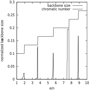
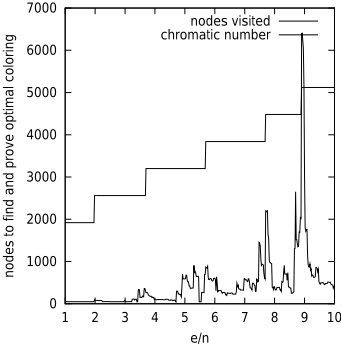
In Figure 1, we plot the frozen development for a typical

50 node graph. Just before the chromatic number increases, there are distinct peaks in backbone size. When the chromatic number increases, the backbone size immediately collapses. In Figure 2, we plot the search cost to find the optimal coloring for the same 50 node graph. To find optimal colorings, we use an algorithm due to Mike Trick which is based upon Brelaz's DSATUR algorithm [Brelaz, 1979]. Search cost peaks with the increases in chromatic number and the peaks in the backbone size. Optimization here closely resembles decision since it is usually not hard to prove that a coloring is optimal. There is thus a strong correlation between backbone size and both optimization and decision cost.

4 Traveling salesperson problem

We next consider the traveling salesperson problem. A leg in a traveling salesperson (TSP) optimization problem is frozen iff it occurs in every possible optimal tour. The TSP backbone is simply the set of frozen legs. We say that the TSP backbone is complete iff it is of size ✂ . In such a situation, the optimal tour is unique. Note that it is impossible to have a backbone of size ✂ ✟ ✡ . It is, however, possible to have a backbone of any size ✂ ✟ ✏ or less. Computing the TSP backbone highlights a connection with sensitivity analysis. A leg occurs in the backbone iff adding some distance, ✢ to the corresponding entry in the inter-city distance matrix increases the length of the optimal tour. A TSP problem with a large backbone is therefore more sensitive to the values in its inter-city distance matrix than a TSP problem with a small backbone.

To explore the development of the backbone in TSP optimization problems, we generated 2-D integer Euclidean problems with ✏ ✖ cities randomly placed in a square of length ✣ . We varied ✤ ✥ ✧ ★ ✆ ✣ ☞ from 2 to 18, generating 100 problems at each integer value of ✤ ✥ ✧ ★ ✆ ✣ ☞ , and found the backbone and the optimal tour using a branch and bound algorithm based on the Hungarian heuristic. The cost of computing the backbone limited the experiment to ✂ ✯ ✏ ✖ . The backbone quickly becomes complete as ✤ ✥ ✧ ★ ✆ ✣ ☞ is increased. Figure 3 is a scatter plot of backbone size against the cost to find and prove the tour optimal.

The Pearson correlation coefficient, ✱ between the normalized backbone size and the log of the number of nodes visited to find and prove the tour optimal is just -0.0615. This suggests that there is a slight negative correlation between backbone size and TSP optimization cost. We took the log of the number of nodes visited as it varies over 4 orders of magnitude. This conclusion is supported by the Spearman rank correlation coefficient, ✲ which is a distribution free test for determining whether there is a monotonic relation between two variables. The data has a Spearman rank correlation of just -0.0147.

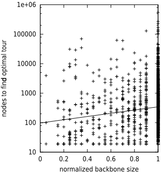
To explore the difference between optimization and decision cost, in Figure 4 we plot the (decision) cost for finding the optimal tour. The Pearson correlation coefficient, ✱ between the normalized backbone size and the log of the number of nodes visited to find the optimal tour is 0.138. This suggests that there is a positive correlation between backbone size and TSP decision cost. This conclusion is supported by the Spearman rank correlation coefficient, ✲ which is 0.126.

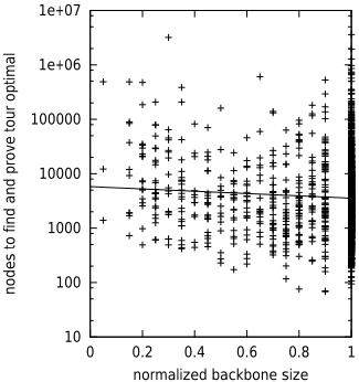
TSP is unlike graph coloring in that optimization appears significantly different from decision. We conjecture this is a result of there usually being no easy proofs of tour optimality. Indeed, the cost of proving tours optimal is negatively correlated with backbone size. This roughly cancels out the positive correlation between the (decision) cost of finding the optimal tour and backbone size. But why does the cost of proving tours optimal negatively correlated with the backbone size? If we have a small backbone, then there are many optimal and near-optimal tours. An algorithm like branch and bound will therefore have to explore many parts of the search space before we are sure that none of the tours is any smaller.

5 Number partitioning

We have seen that whether optimization problems resemble decision problems appears to depend on whether there are cheap proofs of optimality. Number partitioning provides a domain with regions where proofs of optimality are cheap (and there is a positive correlation between optimization cost and backbone size), and regions where proofs of optimality are typically not cheap (and there is a weak negative correlation between optimization cost and backbone size).

One difficulty in defining the backbone of a number partitioning problem is that different partitioning algorithms make different types of decisions. For example, Korf's CKK algorithm decides whether a pair of numbers go in the same bin as each other or in opposite bins [Korf, 1995]. One definition of backbone is thus those pairs of numbers that cannot be placed in the same bin or that cannot be placed in opposite bins. By comparison, the traditional greedy algorithm for number partitioning decides into which bin to place each number. Another definition of backbone is thus those numbers that must be placed in a particular bin. We can break a symmetry by irrevocably placing the largest number in the first bin. Fortunately, the choice of definition does not appear to be critical as we observe very similar behavior in normalized backbone size using either definition. In what follows, we therefore use just the second definition.

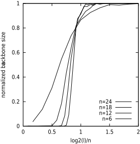
In Figure 5, we plot the frozen development averaged over 100 problems. The frozen development in a single problem is very similar. As in [Gent and Walsh, 1998], we partition ✂ random numbers uniformly distributed in ✵ ✖ ✶ ✣ ☞ . We generate 100 problem instances at each ✂ and ✣ ✹ ✻ ✽ , and then prune numbers to the first ✤ ✥ ✧ ★ ✆ ✣ ☞ bits using mod arithmetic. The size of the optimal partition is therefore monotonically increasing with ✣ . We see characteristic phase transition behaviour ✿ in the backbone size. There is a very sharp increase in backbone size in the region ✖ ❀ ❂ ❃ ✤ ✥ ✧ ★ ✆ ✣ ☞ ✍ ✂ ❃ ✡ where even the best heuristics like KK fail to find backtrack free solutions. By the decision phase boundary at ✤ ✥ ✧ ★ ✆ ✣ ☞ ✍ ✂ ❆ ✖ ❀ ❉ ❊ [Gent and Walsh, 1998], the backbone tends to be complete and the optimal solution is therefore unique. This rapid transition in average backbone size should be compared to graph coloring where [Culberson and Gent, 2000] typically had to look at single instances to see large jumps in backbone size.

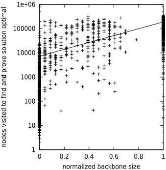
In Figure 6, we give a scatter plot for the optimization cost for Korf's CKK algorithm against backbone size. The data falls into two regions. In the first, optimization problems have backbones less than 80% complete. Optimization in this region is similar to decision as proofs of optimality are typically easy, and optimization cost is positively correlated with backbone size. Data from this region with non-empty backbones has a Pearson correlation coefficient, ✱ of 0.356, and a Spearman rank correlation coefficient, ✲ of 0.388. In the second region, optimization problems have complete backbones. The cost of proving optimality is now typically greater than the cost of finding the optimal solution. Due to the rapid transition in backbone size witnessed in Figure 5, we observed no problems with backbones between 80% and 100% complete.

6 Blocks world planning

Our fourth example taken from the field of planning raises interesting issues about the definition of a backbone. It also highlights the importance of considering the "effective" problem size and of eliminating trivial aspects of a problem.

We might consider a solution to a blocks world planning problem to be the plan and the backbone to be those moves present in all optimal (minimal length) plans. However, since most moves simply put blocks into their goal positions and are therefore trivially present in all plans, almost all of a plan is backbone. A more informative definition results from considering "deadlocks". A deadlock is a cycle of blocks, each of which has to be moved before its successor can be put into the goal position. Each deadlock has to be broken, usually by putting one of the blocks on the table. Once the set of deadlock-breaking moves has been decided, generating the plan is an easy (linear time) problem [Slaney and Thi´ebaux, 1996]. A better definition of solution then is the set of deadlock-breaking moves. However, this is not ideal as many deadlocks contain only one block. These singleton deadlocks give forced moves which inflate the backbone, yet are detectable in low-order polynomial time and can quickly be removed from consideration. We therefore define a solution as the set of deadlock-breaking moves in a plan, excluding those which break singleton deadlocks. The backbone is the set of such moves that are in every optimal solution.

We considered uniformly distributed random blocks world problems of 100 blocks, with both initial and goal states completely specified. To obtain optimal solutions, we used the domain-specific solver reported in [Slaney and Thi´ebaux, 1996] and measured hardness as the number of branches in the search tree. As in [Slaney and Thi´ebaux, 1998], we observed a cost peak as the number of towers in the initial and goal states reaches a critical value of 13-14 towers. We therefore plotted backbone size against the number of towers, and found that this peaks around the same point (see Figure 7).

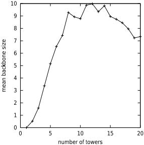
Although problem hardness is in a sense correlated with backbone size, this result must be interpreted carefully because solution size also peaks at the same point. With more than about 13-14 towers, few deadlocks exist so solution size, as we measure it, is small. With a smaller number of towers, the problem instance is dominated by singleton deadlocks, so again the solution is small. The size of the backbone as a proportion of the solution size shows almost no dependence on the number of towers.

Another important feature of the blocks world is that the number of blocks in an instance is only a crude measure of problem "size". At the heart of a blocks world planning problem is the sub-problem of generating a hitting set for a collection of deadlocks. The effective size of an instance is therefore ■ the number of blocks that have to be considered for inclusion in this hitting set. This effective size dominates the solution cost, overshadowing any effect of backbone size. In our next experiment, therefore, we filtered out all but those instances of effective size 35. We obtain similar results restricting to other sizes. Of 9000 random problems, 335 were of effective size 35. For each of those, we measured the hardness of solving two decision problems: whether there exists a plan of length ✣ ❏ ❑ ▼ (the optimal plan length), and whether there exists a plan of length ✣ ❏ ❑ ▼ ✟ ✡ . These can be regarded as measuring the cost of finding an optimal solution and of proving optimality respectively.

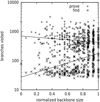
Figure 8 shows the results are similar to TSP problems. Finding an optimal solution tends to be harder if the backbone is larger, for the familiar reason that if solutions are clustered, most of the search space is empty. This data has a Pearson correlation coefficient, ✱ of 0.357 and a Spearman rank correlation coefficient, ✲ of 0.389. Proving optimality, on the other hand, tends to be slightly easier with a larger backbone. This data has ✱ ✯ ✟ ✖ ❀ ✡ ✏ ❊ and ✲ ✯ ✟ ✖ ❀ ✖ ❊ ❂ .

7 Approximation and ❱ -backbones

Our definition of backbone ignores those solutions which are close to optimal. In many real-world situations, we are willing to accept an approximate solution that is close to optimal. We therefore introduce the notion of the ✢ -backbone: the set of frozen decisions in all solutions within a factor ✆ ✡ ✟ ✢ ☞ of optimal. For ✢ ✯ ✖ , this gives the previous definition of backbone. For ✢ ✯ ✡ , the ✢ -backbone is by definition empty. For example, the TSP ✢ -backbone consists of those legs which occur in all tours of length less than or equal to ✣ ❏ ❑ ▼ ✍ ✆ ✡ ✟ ✢ ☞ .

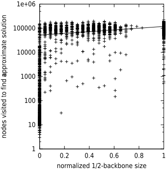
In Figure 9, we give a scatter plot of the size of the ✡ ✍ ✏ - backbone for number partitioning problems against the cost of finding an approximate solution within a factor 2 of optimal. Similar plots are seen for other values of ✢ . As with ✢ ✯ ✖ , the data falls into two regions. In the first, problems have 1/2-backbones less than 80% complete. The cost of approximation in this region is positively correlated with backbone size. However, the correlation is less strong than that between backbone size and optimization cost. Data from this region with non-empty backbones has a Pearson correlation coefficient, ✱ of 0.152, and a Spearman rank correlation coefficient, ✲ of 0.139. In the second region, problems have complete 1/2-backbones. The cost of finding an approximate solutions in this region is now typically as hard as that for the hardest problems with incomplete 1/2-backbones.

8 Related work

First moment methods can be used to show that, at the satisfiability phase transition, the expected number of solutions for a problem is exponentially large. Kamath et al. proved that, whilst most of these problems have few or no solutions, a few have a very large number of clustered solutions [Kamath et al., 1995]. This was verified empirically by Parkes who showed that many variables are frozen although some are almost free [Parkes, 1997]. He argued that such problems are hard for local search algorithms to solve as solutions are clustered and not distributed uniformly over the search space.

Monasson et al. introduced the 2+ ❢ -SAT problem class to study computational complexity in NP-complete decision problems [Monasson et al., 1998]. For ❢ ❃ ❢ ✐ ❆ ✖ ❀ ● ✡ , random 2+❢ -SAT behaves like the polynomial random 2-SAT problem, whilst for ❢ ❧ ❢ ✐ , random 2+ ❢ -SAT behaves like the NP-complete random 3-SAT problem [Monasson et al., 1998; Singer et al., 2000b]. The rapid change in backbone size is continuous (second order) for ❢ ❃ ❢ ✐ , and discontinuous (first ♥ order) for ❢ ❧ ❢ ✐ . This transition may explain the onset of problem hardness and could be exploited in search.

Backbones have also been studied in TSP (approximation) problems [Kirkpatrick and Toulouse, 1985; Boese, 1995]. For example, Boese shows that optimal and near-optimal tours for the well known ATT 532-city problem tended are highly clustered [Boese, 1995]. Heuristic optimization methods for the TSP problem have been developed to identify and eliminate such backbones [Schneider et al., 1996].

A related notion to the backbone in satisfiability is the spine [Bollobas et al., 2001]. A literal is in the spine of a set of clauses iff there is a satisfiable subset in all of whose models the literal is false. For satisfiable problems, the definitions of backbone and spine coincide. Unlike the backbone, the spine is monotone as adding clauses only ever enlarges it.

9 Conclusions

We have studied backbones in optimization and approximation problems. We have shown that some optimization problems like graph coloring resemble decision problems, with problem hardness positively correlated with backbone size and proofs of optimality that are usually easy. With other optimization problems like blocks world and TSP problems, problem hardness is weakly and negatively correlated with backbone size, and proofs of optimality that are usually very hard. The cost of finding optimal and approximate solutions tends, however, to be positively correlated with backbone size. A third class of optimization problem like number partitioning have regions of both types of behavior.

What general lessons can be learnt from this study? First, backbones are often an important indicator of hardness in optimization and approximation as well as in decision problems. Second, (heuristic) methods for identifying backbone variables may reduce problem difficulty. Methods like randomization and rapid restarts [Gomes et al., 1998] may also be effective on problems with large backbones. Third, it is essential to eliminate trivial aspects of a problem, like symmetries and decisions which are trivially forced, before considering its hardness. Finally, this and other studies have shown that there exist an number of useful parallels between computation and statistical physics. It may therefore pay to map over other ideas from areas like spin glasses and percolation.

Acknowledgements

The second author is an EPSRC advanced research fellow. We wish to thank the members of the APES research group.