
A backbone-search heuristic for efficient solving of hard 3-SAT formulae
Proceedings of the Seventeenth International Joint Conference on Artificial Intelligence. Pages 248-252.
© 2001 International Joint Conferences on Artificial Intelligence
Abstract
Of late, new insight into the study of random -SAT formulae has been gained from the introduction of a concept inspired by models of physics, the ‘backbone’ of a SAT formula which corresponds to the variables having a fixed truth value in all assignments satisfying the maximum number of clauses. In the present paper, we show that this concept, already invaluable from a theoretical viewpoint in the study of the satisfiability transition, can also play an important role in the design of efficient DPL-type algorithms for solving hard random -SAT formulae and more specifically -SAT formulae. We define a heuristic search for variables belonging to the backbone of a -SAT formula which are chosen as branch nodes for the tree developed by a DPL-type procedure. We give in addition a simple technique to magnify the effect of the heuristic. Implementation yields DPL-type algorithms with a significant performance improvement over the best current algorithms, making it possible to handle unsatisfiable hard 3-SAT formulae up to 700 variables.
- [Bayardo and Schrag, 1996] R. Bayardo and R. Schrag. Us- ing CSP look-back techniques to solve real-world SAT in- stances. In Proc. of the 14th Nat. Conf. on Artificial Intel- ligence, pages 203-208. AAAI, 1996.
- [Bollobás et al., 2000] B. Bollobás, C. Borgs, J. T. Chayes, J. H. Kim, and D. B. Wilson. The scaling window of the 2- SAT transition. Random Structures and Algorithms, 2000.
- [Boufkhad and Dubois, 1999] Y. Boufkhad and O. Dubois. Length of prime implicants and number of solutions of random ½ ¾ formulae. Theoretical Computer Science, 215 (1-2):1-30, 1999.
- [Crawford and Auton, 1993] J. M. Crawford and L. D. Au- ton. Experimental results on the crossover point in sat- isfiability problems. In Proc. of the 11th Nat. Conf. on Artificial Intelligence, pages 21-27. AAAI, 1993.
- [Davis et al., 1962] M. Davis, G. Logemann, and D. Love- land. A machine program for theorem-proving. Comm. Assoc. for Comput. Mach., (5):394-397, 1962.
- [Dubois et al., 1996] O. Dubois, P. Andre, Y. Boufkhad, and J. Carlier. SAT versus UNSAT. DIMACS Series in Discrete Math. and Theoret. Comp. Sc., pages 415-436, 1996.
- [Freeman, 1996] J. W. Freeman. Hard random 3-SAT prob- lems and the Davis-Putnam procedure. Artificial Intelli- gence, 81(1-2):183-198, 1996.
- [Garey and Johnson, 1979] M. R. Garey and D. S. Johnson. Computers and Intractability / A Guide to the Theory of NP-Completeness. W.H. Freeman & Company, San Fran- cisco, 1979.
- [Gent and Walsh, 1994] I. P. Gent and T. Walsh. The SAT phase transition. In Proc. of the 11th European Conf. on Artificial Intelligence, pages 105-109. ECAI, 1994.
- [Li and Gerard, 2000] C. M. Li and S. Gerard. On the limit of branching rules for hard random unsatisfiable 3-SAT. In Proc. of European Conf. on Artificial Intelligence, pages 98-102. ECAI, 2000.
- [Li, 1999] C. M. Li. A constraint-based approach to narrow search trees for satisfiability. Information Processing Let- ters, 71(2):75-80, 1999.
- [Mitchell et al., 1992] D. Mitchell, B. Selman, and H. J. Levesque. Hard and easy distribution of SAT problems. In Proc. 10th Nat. Conf. on Artificial Intelligence. AAAI, 1992.
- [Monasson et al., 1999] R. Monasson, R. Zecchina, S. Kirk- patrick, B. Selman, and L. Troyansky. Determining com- putational complexity from characteristic 'phase transi- tions'. Nature 400, pages 133-137, 1999.
- [Selman et al., 1997] B. Selman, H. Kautz, and D. McAllester. Ten challenges in propositional rea- soning and search. In Proc. of IJCAI-97, 1997. IJCAI
- [Zhang, 1997] H. Zhang. SATO. an efficient propositional prover. In Proc. of the 14th Internat. Conf. on Automated Deduction, pages 272-275. CADE-97, LNCS, 1997.
References were extracted automatically from the PDF and may contain errors.
Full text extracted automatically from the PDF; figures, tables and equations may differ. The PDF is the version of record.
1 Introduction
The Satisfiability Problem, as one of the basic NP-complete problems [Garey and Johnson, 1979], has appeared to possess a property of great interest with respect to computational complexity. Random CNF formulae in which each clause has a fixed number ✄ of literals, known as ✄ -SAT formulae, exhibit with respect to satisfiability, a so-called phase transition phenomenon such that the SAT formulae at the transition appear in probability the most difficult to solve. This property, initially described in [Mitchell et al., 1992] and since studied in numerous papers [Crawford and Auton, 1993; Gent and Walsh, 1994] has the following practical manifestation. When in an experiment ✆ clauses with exactly ✄ literals, ✄ ✝ ✟ , ☎ , ✡ ... (limited to manageable sizes of formulae), over a set of ☛ boolean variables, are chosen at random with a fixed ratio ☞ ✝ ✆ ✎ ☛ , the probability of satisfiability falls abruptly from near ✒ to near ✓ as ☞ passes some critical value called the threshold. Moreover (leaving aside 2-SAT
✔ This work was supported by Advanced Micro Devices Inc.
formulae which are well known to be solvable in polynomial time), at the threshold, for ✄ ✕ ☎ a peak of difficulty of solving is observed and this peak grows exponentially as a function of ☛ . This intriguing property correlating the satisfiability threshold with the hardness of ✄ -SAT formulae, has stimulated many theoretical as well as experimental studies, eliciting a better understanding of the phase transition phenomenon and progress in solving hard SAT formulae.
Recently, the satisfiability phase transition has attracted much attention from physicists. Sophisticated models of statistical physics have been evolved over the past few decades to predict and analyze certain phase transitions, and these can be compared, from a theoretical viewpoint, with the satisfiability transition. This has shed new light on the question. In particular in 1999, an insightful concept was introduced, the 'backbone' of a SAT formula [Monasson et al., 1999]. The backbone corresponds to the set of variables having a fixed truth value in all assignments satisfying the maximum number of clauses of a ✄ -SAT formula (cf MaxSAT). The relevance of this concept is connected to the fact that the number of solutions (i.e. satisfying assignments) of a satisfiable random ✄ - SAT formula has been proved to be almost surely exponential as a function of ☛ up to and at the threshold [Boufkhad and Dubois, 1999], a result corroborated in its MaxSAT version by the physics model known as 'Replica Symmetric ansatz'. This concept of backbone of a ✄ -SAT formula has turned out to play an important role in theoretical studies, allowing for example, the scaling window of the 2-SAT transition to be determined [Bollob´as et al., 2000]. We show in this paper that the concept of backbone can also play an important role in more efficiently solving hard ✄ -SAT formulae. We will focus particularly on 3-SAT formulae which are the easiest ✄ -SAT formulae to handle (for ✄ ✕ ☎ ) and therefore at present the most studied in the literature. The hard 3-SAT formulae are generated randomly with a ratio ☞ around ✡ ✚ ✟ ✜ which appears experimentally to be close to the threshold value. In the last ten years, the best-performing complete solving algorithms (i.e., those definitely determining whether a solution exists or not) have been based on the classical DPL procedure [Davis et al., 1962]. Important progress was achieved, making it possible at present, for example, to solve ☎ -SAT hard formulae with 300 variables (and therefore with 1275 clauses) in roughly the same computing time as formulae with 100 variables (and 425 clauses) ten years ago under equivalent computing conditions.
The DPL-type procedures which have led to this progress were all designed according to a single viewpoint, that of dealing with the clauses which remain not satisfied at successive nodes of the solving tree, trying mainly to reduce them as much as possible in number and in size. Clauses already satisfied in the course of solving were not considered. By using the concept of backbone we change this viewpoint, focusing on the clauses which can be satisfied in the course of solving, and how. Thus, we first explain in this paper how with this new viewpoint, the size of trees developed by a DPL-type procedure can be efficiently reduced. Then we give practically a simple branching heuristic based on the search for variables belonging to the backbone of a formula, and we show that it brings immediately an improvement in performance compared with the best current heuristic, this improvement increasing with the number of variables. We further present a technique to magnify the effect of the heuristic. Combining this heuristic and this technique in a DPL-type procedure, we obtain significant performance improvements over existing SAT solvers in the literature, solving unsatisfiable hard random 3-SAT formulae with 200 to 600 variables from 1.2 to about 3 times faster than by the current best suitable algorithms, particularly satz214 [Li, 1999]. Moreover, hard 3-SAT formulae up to 700 variables are shown to be solvable by our procedure in about 25 days of computing time, which begins to be relatively acceptable. These experimental results reported in the present paper bring an up beat view in contrast to the misgivings expressed in [Li and Gerard, 2000] about the possibility to obtain further significant progress with DPL-type algorithms, which went as far as to suggest that the best current algorithms could be close to their limitations.
2 An approach using the concept of backbone for designing efficient DPL-type procedures.
In this section, we need to generalize the notion of backbone of a SAT formula ✣ . Given a set of clauses ✤ , no longer necessarily of maximum size, we define the backbone associated to ✤ as the set of literals of ✣ having the truth value TRUE in all assignments satisfying the clauses of ✤ .
Since the overall performance of a complete algorithm on random SAT formulae depends essentially on how it handles unsatisfiable formulae, in the remainder of this section we consider only unsatisfiable 3-SAT formulae. Let, then, ✣ be an unsatisfiable 3-SAT formulawith clauses built on a set ✥ of ✟ ☛ literals, itself derived from a set ✧ of ☛ boolean variables. Let ★ be the so-called refutation tree of ✣ , as developed by a DPL-type procedure. At each leaf ✩ of ★ , an inconsistency is detected. Let ✪ ✫ ✩ ✭ be the subset of clauses of ✣ satisfied by the ✯ ✫ ✩ ✭ literals set to TRUE along the path ✱ ✫ ✩ ✭ from the root of ★ to the leaf ✩ . Call ✳ ✫ ✩ ✭ the set of assignments satisfying ✪ ✫ ✩ ✭ . Suppose there is a backbone ✶ ✫ ✩ ✭ associated to ✪ ✫ ✩ ✭ . From the above-mentioned theoretical study, this can be expected in practice often to be the case at the leaves of ★ . The inconsistency detected at ✩ means that ✟ ✸ ✺ ✼ ✾ ❀ ❂ assignments are refuted as possible solutions of ✣ . We have the inequality: ✟ ✸ ✺ ✼ ✾ ❀ ❂ ❄ ❆ ✳ ✫ ✩ ✭ ❆ . Equality obtains precisely when the set of the ✯ ✫ ✩ ✭ literals constitutes the backbone ✶ ✫ ✩ ✭ of ✪ ✫ ✩ ✭ . Furthermore, the assignments refuted as possible solutions of ✣ at different leaves of ★ are distinct (form disjoint sets), and their total number equals ✟ ✸ . Hence, in lowering the number of leaves of ★ two factors intervene, namely: (i) the size of the sets ✳ ✫ ✩ ✭ must be as large as possible, and (ii) the equality ✟ ✸ ✺ ✼ ✾ ❀ ❂ ✝ ❆ ✳ ✫ ✩ ✭ ❆ must hold most of the time, at least approximately.
The above considerations extend to all nodes of ★ . In this case, at any node ■ , ✟ ✸ ✺ ✼ ✾ ❏ ❂ represents the potential maximum number of assignments that can be refuted as possible solutions of ✣ at the node ■ . According to the above viewpoint, the global condition in order best to reduce the size of ★ is that, from the root to a nearest node ■ , literals be chosen which constitute a backbone relative to some subset of clauses of ✣ . Indeed, the nearer the node ■ is to the root, the smaller the set ✪ ✫ ■ ✭ of satisfied clauses will tend to be. Now, the crucial point is that any assignment giving the value FALSE to at least one literal of the backbone, can be refuted on the basis of the subset ✪ ✫ ■ ✭ of clauses associated to ✶ ✫ ■ ✭ . If the set ✪ ✫ ■ ✭ is of small size, it is then to be expected that any refutation derived from ✪ ✫ ■ ✭ be short, i.e. that the refutation tree for all such assignments be of small size. Let us illustrate this with the following very simple example. Suppose that among all the clauses of ✣ there are 4 of the form: ❖ ✫ a80 ❘ ❚ ❘ ❱ ✭ ❲ ✫ a80 ❘ ❚ ❘ ❱ ✭ ❲ ✫ a80 ❘ ❚ ❘ ❩ ✭ ❲ ✫ a80 ❘ ❚ ❘ ❩ ✭ ❪ . The backbone of these 4 clauses reduces to the literal a80 . According to the above principle, this literal is a preferential choice for a branch stemming from the root. In the branch of the literal a80 , refutations are obtained by branching just twice, applying the same principle of bringing forward a backbone at the nearest possible node, thus either ❚ or ❚ will be chosen indifferently. Note that in this example the backbone search principle includes in its general form the notion of resolvent without using it. The literal a80 could of course be inferred by applying classical resolution.
We next detail a heuristic and a technique which embody the foregoing, if only partially.
2.1 A backbone-variables search heuristic
Consider a generic node ■ of the refutation tree ★ of ✣ , and let ✣ ✫ ■ ✭ be the reduced formula at node ■ . The heuristic (Figure 1) described below aims at selecting literals that may belong to a hypothetical backbone associated to a subset of clauses of ✣ of the smallest possible size. The simple idea sustaining this heuristic is to estimate the number of 'possibilities' for a given literal ❩ of ✣ ✫ ■ ✭ to be constrained to TRUE in the clauses of ✣ ✫ ■ ✭ where it appears. E.g., if ✣ ✫ ■ ✭ contains the clause ✫ ❩ ❘ ❵ ❘ ❜ ✭ , one possibility for ❩ to be TRUE is ✫ ❵ ❘ ❜ ✭ ❝ ✣ ✤ ✥ ✳ ❤ . If in addition ❵ and ❜ appear ❥ and ❦ times, respectively, in clauses of ✣ ✫ ■ ✭ , the number of possibilities for ❩ to be TRUE can be estimated as ❥ ❦ at this second level by setting to FALSE the necessary literals in the clauses where ❵ and ❜ appear. If however ❵ and ❜ appear in both binary and ternary clauses, we must consider the possibility to be greater when a binary rather than a ternary clause is involved, since a single literal is required to have the value FALSE instead of two. To evaluate a 'possibility', we therefore weight the relevant binary and ternary clauses. But for Set ❧ ♠ ✓ and let MAX be an integer. Proc ♣ ✫ ❩ ✭ ❧ ♠ ❧ a115 ✒ compute ✈ ✫ ❩ ✭ if ❧ ① MAX then Return ② ✾ ③ ④ ⑤ ❂ ⑥ ⑧ ✾ ⑨ ❂ ♣ ✫ ❵ ✭ ♣ ✫ ❜ ✭ else Return ② ✾ ③ ④ ⑤ ❂ ⑥ ⑧ ✾ ⑨ ❂ ✫ ✟ ❥ ❺ ✫ ❵ ✭ a115 ❥ ❼ ✫ ❵ ✭ ✭ ✫ ✟ ❥ ❺ ✫ ❜ ✭ a115 ❥ ❼ ✫ ❜ ✭ ✭
end if
Figure 1: backbone search heuristic h
the heuristic evaluation, only the ratio of the weightings matters. As a first apporximation, we take the ratio of probabilities in a random assignment, i.e. simply a ratio of 2. Within the heuristic function, an evaluation level is defined for ❩ , as exemplified by the above allusion to a second-level evaluation of ❩ . To be precise, the evaluation level is the number of ternary clauses which must successively be brought into play in order to reach the conclusion that ❩ is TRUE, following the aforementioned principle. Fixing an evaluation level thus limits the number of ternary clauses to be used before concluding that ❩ is TRUE. On the other hand, there is no need to limit the number of binary clauses that can be used, with or without ternary ones. Since binary clauses, due to the fact that a single literal has to be FALSE, do not give rise to combinations, their use does not increase the computational complexity of the heuristic. At a given node of the refutation tree, all literals must be evaluated to the same level so as to guarantee comparable evaluations. The heuristic function ♣ in Figure 1 embodies the simple principles just stated. The estimation level equals the number of recursive calls to ♣ ✫ ❩ ✭ , namely the constant MAX augmented by 1. For the formal definition of the heuristic, there remains to introduce two types of sets of clauses. ❽ ✫ ❩ ✭ denotes the set of binary or unary clauses derived by eliminating ❩ , from the clauses of ✣ ✫ ■ ✭ where ❩ appears. Let ❥ ❺ ✫ ❵ ✭ and ❥ ❼ ✫ ❵ ✭ be the number of unary and binary clauses respectively in ❽ ✫ ❵ ✭ . ✈ ✫ ❩ ✭ is the set of all binary subclauses derived from ternary clauses of ✣ ✫ ■ ✭ such that each of these binary subclauses set to FALSE, implies ❩ TRUE either directly or by virtue of certain unary clauses having the value FALSE. Let us take an example showing how to compute the heuristic h. Consider the following set of clauses:
✫ a80 ❘ ❾ ❘ ❿ ✭ ➀ ✫ a80 ❘ ☞ ✭ ➀ ✫ ☞ ❘ ➂ ❘ ➃ ✭ ➀ ✫ ❾ ❘ ➅ ❘ ➂ ✭ ➀ ✫ ❾ ❘ ➇ ✭ ➀ ✫ ❿ ❘ ➅ ❘ ➇ ✭ ➀ ✫ ➂ ❘ ➃ ✭ .
We evaluate ♣ ✫ a80 ✭ on the above set of clauses with MAX set to 1. We have ✈ ✫ a80 ✭ ✝ ❖ ❾ ❘ ❿ ➌ ➂ ❘ ➃ ❪ . To carry out the evaluation, the sets ❽ ✫ ❵ ✭ must be determined for each literal ❵ appearing in the clauses of ✈ ✫ a80 ✭ , in order to know the values ❥ ❺ ✫ ❵ ✭ and ❥ ❼ ✫ ❵ ✭ . We thus have: ❽ ✫ ❾ ✭ ✝ ❖ ➅ ❘ ➂ ➌ ➇ ❪ , ❽ ✫ ❿ ✭ ✝ ❖ ➅ ❘ ➇ ❪ , ❽ ✫ ➂ ✭ ✝ ❖ ➃ ➌ ❾ ❘ ➅ ❪ and ❽ ✫ ➃ ✭ ✝ ❖ ➂ ❪ . With regard to ❽ ✫ ❾ ✭ , we have ❥ ❺ ✫ ❾ ✭ ✝ ✒ because of the unary clause ➇ , and ❥ ❼ ✫ ❾ ✭ ✝ ✒ owing to ➅ ❘ ➂ . Proceeding thus for all variables in the clauses of ✈ ✫ a80 ✭ , the value of ♣ ✫ a80 ✭ is :
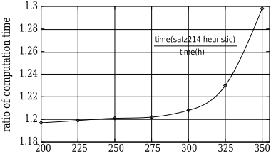
We assessed the performance of the heuristc ♣ ✫ ❩ ✭ in a pure DPL procedure. At each node of the tree developed by the procedure, the product ♣ ✫ a80 ✭ ♣ ✫ a80 ✭ was computed for every as yet unassigned variable a80 . The chosen branching variablewas that corresponding to the maximum value of ♣ ✫ a80 ✭ ♣ ✫ a80 ✭ at the node under consideration. The product ♣ ✫ a80 ✭ ♣ ✫ a80 ✭ favors opposite literals which may each belong to a different backbone relative to a separate subset of clauses. The performance of this heuristic was compared to that of a heuristic of the type used in recent algorithms. We implemented the heuristic of the solver "satz214" [Li, 1999], appearing currently to be the fastest for solving random 3-SAT formulae. We solved samples of 200 random 3-SAT formulae having from 200 to 300 variables in steps of 25, and a clauses-to-variables ratio of 4.25. For every considered number of variables, the mean ratio of the computation time with the satz214 heuristic compared to the computation time with the heuristic described above ("h" heuristic), for a level limited to 3, has been plotted on Figure 2. The smooth line connecting the consecutive points shows the evolution of this mean ratio from 200 to 300 variables. This ratio is seen to be markedly above 1, it increases from 1.2 to 1.3 with accelerated growth. Table 1
size of hard random unsatisfiable problem (in #variables)
Figure 2: mean time ratio of satz214 heuristic to "h" heuristic on hard random 3-SAT unsatisfiable formulae.
gives the mean size of the tree developed with either heuristic. These results immediately demonstrate the advantage of the approach based on the concept of backbone.
| size of formulae in #vars | "↕ " heuristic mean #nodes | satz214 heuristic mean #nodes |
|---|---|---|
| 200 | 1556 | 1647 |
| 225 | 3165 | 3363 |
| 250 | 8229 | 8774 |
| 275 | 18611 | 20137 |
| 300 | 36994 | 41259 |
| 325 | 77744 | 93279 |
| 350 | 178813 | 252397 |
2.2 Picking backbone variables
The technique described in this section aims at improving the efficiency of the previous heuristic by detecting either literals which must belong to some backbone relative to some set of clauses, or clauses that cannot be associated to literals belonging to a backbone. Only the principles of the technique are given in this section, together with illustrative examples. A literal ❩ has to belong to a backbone relative to some set of clauses, if among all possibilities leading to ❩ being TRUE, at least one will necessarily hold. Take the simple example of the following clauses:
Example 1:
Consider the literal a80 . At the first level, the possibilities that it be true are ✫ ➇ ❘ ♣ ❝ ✣ ✤ ✥ ✳ ❤ ✭ and ✫ ❿ ❘ ☞ ❝ ✣ ✤ ✥ ✳ ❤ ✭ . At the second level, these possibilities become simply ❾ ❝ ✣ ✤ ✥ ✳ ❤ and ❾ ❝ ✣ ✤ ✥ ✳ ❤ . Necessarily one or the other will obtain. Therefore, a80 belongs to the backbone associated to the given set of clauses.
Conversely, a literal ❩ in some clause cannot belong to a backbone, if setting to TRUE, it leads to an inconsistency. This principle generalizes the classical local treatment of inconsistency detection at each node of a solving tree, such as implemented in csat, posit, and satz214. As an example, take the following clauses:
Example 2:
According to the criteria usually adopted by algorithms in the literature, only the literal a80 or at most the 2 literals a80 and a80 in the clauses of Example 2 will be selected for a local treatment of inconsistency detection. Setting a80 to TRUE leads to an inconsistency by unit propagation. From the backbone viewpoint, a80 cannot, therefore, belong to a backbone. As mentioned, this case is classically handled by existing algorithms. Now suppose that, instead of the sixth clause ✫ ➃ ❘ ❾ ✭ we have the clause ✫ ➃ ❘ ❾ ❘ ➜ ✭ . Unit propagation no longer detects an inconsistency. On the other hand, following our backbone viewpoint and without changing the classical selection criteria for the local treatment of inconsistencies (which are of recognized efficiency), it is possible to detect that the first clause containing a80 , ✫ a80 ❘ ➜ ✭ , cannot contribute to a set of clauses such that a80 would belong to a backbone relative to this set. Indeed, the only possibility that a80 be TRUE is that ➜ be FALSE. An inconsistency now follows, again by unit propagation. As a consequence, ➜ is set to TRUE, and the clause ✫ a80 ❘ ➜ ✭ cannot be associated to a backbone including a80 . The technique inspired by the principle just stated is called pickback.
We briefly mention two other examples which show the general nature of this principle.
Example 3:
Setting a80 to TRUE does not lead to an inconsistency. Yet, setting ✫ ➜ ❘ ➟ ✭ to FALSE by 'pickback' leads, via unit propagation, to an inconsistency. We may therefore add this clause,
✫ ➜ ❘ ➟ ✭ , which subsumes ✫ a80 ❘ ➜ ❘ ➟ ✭ .
Example 4:
Setting a80 to TRUE does not lead to an inconsistency. Yet setting ➜ alone to FALSE in ✫ ➜ ❘ ➟ ✭ allows to deduct the value FALSE for ➟ , thus validating a stronger pickback than in the previous example.
3 Experimental results
The "h" heuristic and the technique just described in section 2 were implemented in a DPL procedure. This implementation is denoted cnfs (short for CNF solver). In this section comparative performance results are given, pitting cnfs against 4 solvers which currently appear to be the best performers on ✄ -SAT or ☎ -SAT random formulae. These are: TABLEAU in its version ntab [Crawford and Auton, 1993], posit [Freeman, 1996], csat [Dubois et al., 1996], and satz214 1 [Li, 1999]. In addition we consider 2 strong solvers sato [Zhang, 1997], rel sat [Bayardo and Schrag, 1996] which are more devoted to structured formulae than to random formulae. We carried out our experimentations on random 3-SAT formulae generated as per the classical generators in the literature (i.e. each clause drawn independently and built by randomly drawing 3 among a fixed number ☛ of variables, then negating each with probability ❺ ❼ ). In order that the impact of the backbone approach used in cnfs be shown with as much precision as possible, our experiments covered a wide range of formula sizes, going from 200 to 700 variables and drawing large samples. The hardware consisted of AMD Athlon-equipped 2 PCs running at 1 GHz under a Linux operating system. The comparative results thus obtained are now to be given in detail.
3.1 Performance comparison results
Comparative results from 200 to 400 variables
Table 2 gives the mean sizes of the solving trees developed by the 7 programs under scrutiny, sato, rel sat, ntab, csat, posit, satz214 and cnfs, on samples of 1000 formulae with 200 and 300 variables, and on samples of 500 formulae with 400 variables. Mean tree sizes are expressed as numbers of branching nodes, and are listed separately for satisfiable and unsatisfiable formulae. They are found to be from 8 to about 1.5 times smaller for cnfs than for the 4 solvers ntab, csat, posit and satz214 in the case of unsatisfiable formulae, and from 9 to 1.6 times smaller for satisfiable formulae; these ratios depend on both solver and formula size. It is important to observe that the compute time ratio of cnfs with respect to each of the other 6 solvers increases with formula size. Table 3 shows how improved tree sizes obtained with cnfs translate into computation times. Compute time ratios of cnfs with respect to ntab, csat, posit and satz214 are seen to vary from 26 to 1.3 in the unsatisfiable, and from 29 to 1.75 in the satisfiable case. Tree size improvements thus carry over into equivalent computation time gains. These first results show, therefore, that cnfs provides, in the range of formulae from
1 The new satz215 has, from our first experiments, similar performances on Random 3-SAT formulae as satz214
2 Advanced Micro Devices Inc. (http://www.amd.com)
| SAT Solvers | unsat (N) & sat (Y) | 200 V 850 C (482 N) (518 Y) mean #nodes (std dev.) | 300 V 1275 C (456 N) (534 Y) mean #nodes (std dev.) | 400 V 1700 C (245 N) (255 Y) mean #nodes in millions (std dev.) |
|---|---|---|---|---|
| sato | unsat sat | 14076 (5225) 4229 (4754) | 443313 (109694) 151728 (157102) | - - |
| rel sat | unsat sat | 1319 (535) 478 (452) | 56064 (26136) 18009 (19217) | 2.2 (0.9) 0.82 (0.88) |
| ntab | unsat sat | 973 (764) 756 (673) | 78042 (33222) 27117 (27790) | 3.0 (1.4) 1.1 (1.2) |
| csat | unsat sat | 2553 (997) 733 (763) | 90616 (37729) 26439 (31224) | 3.6 (1.7) 1.8 (2.4) |
| posit | unsat sat | 1992 (754) 789 (694) | 82572 (35364) 34016 (31669) | 3.4 (1.7) 1.5 (1.4) |
| satz214 | unsat sat | 623 (206) 237 (216) | 18480 (7050) 6304 (6541) | 0.56 (0.23) 0.21 (0.21) |
| cnfs | unsat sat | 470 (156) 149 (154) | 12739 (4753) 3607 (4089) | 0.37 (0.15) 0.12 (0.13) |
200 to 400 variables, significant performance improvements that increase with formula size, in terms of tree size as well as computation time.
Further performance comparisons with satz214
Pursuing this line of experimentation, we now offer performance comparison results on formulae from 400 to 600 variables with the satz214 solver, which performs best of the 6 against which cnfs was measured up to now.
We first solved samples of 100 formulae from 400 to 600 variables in increments of 20.
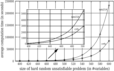
Figure 3: mean computation time of satz214 & cnfs on 3-SAT hard random unsatisfiable formulae from 400 to 600 variables
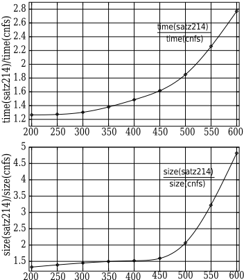
ted in the same way as for the Figure 2) of satz214 and cnfs for the unsatisfiable formulae within the solved samples. Indeed, the most significant performance figure for a complete algorithm is on unsatisfiable formulae. The gain previously observed between 200 and 400 variables is seen further to increase from 400 to 600. cnfs is 1.85 times faster than satz214 for 500 variables, and 2.78 times faster for 600.
| SAT Solvers | unsat (N) & sat (Y) | 200 V 850 C (482 N) (518 Y) mean time (std dev.) | 300 V 1275 C (456 N) (534 Y) mean time (std dev.) | 400 V 1700 C (245 N) (255 Y) mean time (std dev.) |
|---|---|---|---|---|
| sato | unsat sat | 89.2s (84.6s) 13.2s (38s) | 18h 27m (7h) 4h (6h 40m) | - - |
| rel sat | unsat sat | 4.5s (1.9s) 1.6s (1.6s) | 343s (169s) 114.3s (123s) | 6h 29m (2h 47m) 2h 30m (2h 40m) |
| ntab | unsat sat | 0.81s (0.30s) 0.38s (0.28s) | 48.0s (20.6s) 16.6s (16.8s) | 48m 15s (23m 21s) 18m 5s (19m 16s) |
| csat | unsat sat | 0.47s (0.20s) 0.15s (0.15s) | 29.6s (13.3s) 9.0s (10.7s) | 29m 1s (14m 36s) 7m 47s (10m 1s) |
| posit | unsat sat | 0.28s (0.1s) 0.11s (0.1s) | 15.1s (6.6s) 6.3s (5.9s) | 13m 7s (6m 35s) 5m 56s (5m 36s) |
| satz214 | unsat sat | 0.17s (0.05s) 0.07s (0.05s) | 4.9s (1.8s) 1.7s (1.7s) | 2m 44s (1m 09s) 1m 05s (1m 03s) |
| cnfs | unsat sat | 0.13s (0.04s) 0.04s (0.04s) | 3.7s (1.3s) 1.1s (1.2s) | 1m 50s (0m 43s) 0m 37s (0m 40s) |
| #Vars #Clauses | unsat (N) sat (Y) | mean #nodes in millions (std dev.) | mean time (std dev.) | ||
|---|---|---|---|---|---|
| cnfs | satz214 | cnfs | satz214 | ||
| 500 V | ➠ ➡ N | 8 (3.3) | 16.6 (7.2) | 49m 10s (19s) | 91m 02s (39s) |
| 2125 C | ➢ ➤ Y | 2.5 (3.8) | 6.5 (7.2) | 15m 24s (23s) | 36m 21s (40s) |
| 600 V | ➥ ➡ N | 178 (71) | 857 (373) | 23h 18m (9h) | 64h 32m (28h) |
| 2550 C | ➠ ➤ Y | 37.8 (50) | 233 (315) | 4h 54m (6.5h) | 18h 20m (24h) |
Table 4: average size of tree and mean computation time on hard random 3-SAT formulae from 500 and 600 variables
and computation time on formulae with 500 and 600 variables, listing the satisfiable and unsatisfiable cases separately. Tree size gain increase of cnfs versus satz214 may be noticed not to carry over entirely into computation time gain increase. Indeed, the gain factor for cnfs on unsatisfiable formulae goes from 2 for 500 variables to 4.8 for 600. This probably reflects the high cost of the backbone-variable search heuristic. One can therefore hope that technical improvements of the latter will lead to yet greater computation time performance gains. Finally, Figure 4 sums up, on the whole range 200 to 600 variables, the evolution of the gain ratio of cnfs vs satz214 in computation time and tree size. These curves clearly demonstrate a complexity function gain of cnfs over sat214 on random 3-SAT formulae.
Solving hard 3-SAT formulae up to 700 variables
For the reader's information, Table 5 shows how cnfs performs in computation time and number of nodes on two samples of 30 formulae with 650 and 700 variables, respectively. Formulae with 700 variables, regarded as quite large for complete solving methods [Selman et al., 1997] are now within reach, and this in approximately 600 machine hours on a single-processor 'domestic' PC. Let us also indicate that for random formulae with 700 variables, irrespective of their satisfiability, the mean solving time with cnfs is about 300 hours.
200
250
300
350
400
size of hard random unsatisfiable problem (in #variables)
| #Vars #Clauses | unsat (N) sat (Y) | mean #nodes in millions (std dev.) | mean time (std dev.) |
|---|---|---|---|
| 650 V | ➸ ➺ N | 1140 (587) | 5 days 21h (71h) |
| 2762 C | ➸ ➻ Y | 241 (399) | 1 day 6h (50h) |
| 700 V | ➸ ➤ N | 4573 (1703) | 26 days 4h (228h) |
| 2975 C | ➸ ➡ Y | 653 (922) | 3 days 19h (129h) |
Table 5: mean computation time and average size of tree of cnfs on large hard 3-SAT formulaes up to 700 variables
4 Conclusion
In the course of the last decade, algorithms based on the DPL procedure for solving propositional formulae have seen a performance improvement that was quite real, if much less spectacular than in the case of stochastic algorithms. It was recently suggested that the performance of DPL-type algorithms might be close to their limitations, giving rise to a fear that subsequent progress might be very difficult to achieve and that large unsatisfiable formulae (e.g., 700 variables) might remain beyond reach. We have presented a DPL-type algorithm incorporating mainly a new and simple heuristic using the backbone concept recently introduced from models of physics. This concept has changed the viewpoint from which classical heuristics were developed. We were thus able to improve the current best solving performance for hard 3SAT formulae by a ratio increasing with formula size (equal to 3 for 600 variables), and we have shown that solving unsatisfiable formulae with 700 variables was feasible. An important lesson can be drawn from our results. In order to improve the performance of DPL-type algorithms significantly and to enhance the state of the art in complete solving, it appears that a deep understanding of the structure of the solutions of a SAT formula is paramount. This is why experimental, as well as theoretical studies aiming to further such comprehension are essential.
@inproceedings{ijcai2001p35,
  title     = {A backbone-search heuristic for efficient solving of hard 3-SAT formulae},
  author    = {Dubois, Olivier and Dequen, Gilles},
  booktitle = {Proceedings of the Seventeenth International Joint Conference on
               Artificial Intelligence, {IJCAI-01}},
  publisher = {International Joint Conferences on Artificial Intelligence},
  editor    = {Bernhard Nebel},
  pages     = {248--252},
  year      = {2001},
  url       = {https://ijcai.org/proceedings/2001/35},
}
TY - CPAPER TI - A backbone-search heuristic for efficient solving of hard 3-SAT formulae AU - Dubois, Olivier AU - Dequen, Gilles T2 - Proceedings of the Seventeenth International Joint Conference on Artificial Intelligence, IJCAI-01 PB - International Joint Conferences on Artificial Intelligence PY - 2001 SP - 248 EP - 252 UR - https://ijcai.org/proceedings/2001/35 ER -Copied
Machine-readable versions of this paper, for tools and AI agents:





