
Cooperative Search and Nogood Recording
Proceedings of the Seventeenth International Joint Conference on Artificial Intelligence. Pages 260-264.
© 2001 International Joint Conferences on Artificial Intelligence
Abstract
Within the framework of constraint satisfaction problem, we propose a new scheme of cooperative parallel search. The cooperation is realized by exchanging nogoods (instantiations which can’t be extended to a solution). We associate a process with each solver and we introduce a manager of nogoods, in order to regulate exchanges of nogoods. Each solver runs the algorithm Forward-Checking with Nogood Recording. We add to algorithm a phase of interpretation, which limits the size of the search tree according to the received nogoods. Solvers differ from each other in ordering variables and/or values by using different heuristics. The interest of our approach is shown experimentally. In particular, we obtain linear or superlinear speed-up for consistent problems, like for inconsistent ones, up to about ten solvers.
- [Bessière and Régin, 1996] C. Bessière and J.-C. Régin. MAC and Combined Heuristics : Two Reasons to Forsake FC (and CBJ?) on Hard Problems. In Proc. of CP 96, pages 61-75, 1996.
- [Clearwater et al., 1991] S. Clearwater, B. Huberman, and T. Hogg. Cooperative Solution of Constraint Satisfaction Problems. Science, 254:1181-1183, Nov. 1991.
- [Hogg and Huberman, 1993] T. Hogg and B. A. Huberman. Better Than the Best: The Power of Cooperation. In L. Nadel and D. Stein, editors, 1992 Lectures in Complex Systems, volume V of SFI Studies in the Sciences of Com- plexity, pages 165-184.
- [Hogg and Williams, 1993] T. Hogg and C.P. Williams. Solving the Really Hard Problems with Cooperative Search. In Proc. of AAAI 93, pages 231-236, 1993.
- [Hogg and Williams, 1994] T. Hogg and C.P. Williams. Ex- pected Gains from Parallelizing Constraint Solving for Hard Problems. In Proc. of AAAI 94, pages 331-336, Seat- tle, WA, 1994.
- [Martinez and Verfaillie, 1996] D. Martinez and G. Verfail- lie. Echange de Nogoods pour la résolution coopérative de problèmes de satisfaction de contraintes. In Proc. of CNPC 96, pages 261-274, Dijon, France, 1996. In french.
- [Schiex and Verfaillie, 1993] T. Schiex and G. Verfaillie. Nogood Recording for Static and Dynamic Constraint Sat- isfaction Problems. In Proc. of the 5¼ 6½ IEEE ICTAI, 1993.
- [Terrioux, 2001] C. Terrioux. Cooperative search and no- good recording. Research report, LIM, 2001.
References were extracted automatically from the PDF and may contain errors.
Full text extracted automatically from the PDF; figures, tables and equations may differ. The PDF is the version of record.
1 Introduction
In constraint satisfaction problems, one of main tasks consists in determining whether there exists a solution, i.e. an instantiation of all variables which satisfies all constraints. This task is a NP-complete problem. In order to speed up the resolution of problems, parallel searches are used. A basic one is independent parallel search which consists in running several solvers (each one using a different heuristic) instead of a single solver. The aim is that at least one of the solvers gets an heuristic suitable for the problem which we solve. Tested on the graph coloring problem ([Hogg and Williams, 1994]), this approach has better results than a classical resolution with a single solver, but the gains seem limited. Hogg and Williams recommend then the use of a cooperative parallel search.
A cooperative parallel search is based on the same ideas as the independent search with in addition an exchange of informations between solvers, in order to guide solvers to a solution, and then, to speed up the resolution. Experimental results on cryptarithmetic problems ([Clearwater et al., 1991; Hogg and Huberman, 1993]) and on graph coloring problem ([Hogg and Huberman, 1993; Hogg and Williams, 1993]) show a significant gain in time with respect to an independent search. In both cases, the exchanged informations correspond to partial consistent instantiations.
In [Martinez and Verfaillie, 1996], a cooperation based on exchanging nogoods (i.e. instantiations which can't be extended to a solution) is proposed. Exchanged nogoods permit solvers to prune their own search tree. So, one can expect to find more quickly a solution. Solvers run the algorithm Forward Checking with Nogood Recording (noted FC-NR [Schiex and Verfaillie, 1993]). The realized implementation gathers all solvers in a single process which simulates the parallelism. It is turned to a monoprocessor system. Experimentations on random CSPs show that cooperative search is better than independent one. However, the weak gain with report to a single solver gives a doubt about efficiency of a such search.
From the idea of Martinez and Verfaillie, we define a new scheme of cooperation with exchange of nogoods, turned to systems with one or several processors. We associate a process with each solver. Each solver runs FC-NR. In order to avoid problems raised by the cost of communications, we introduce a manager of nogoods whose role is to regulate exchange of nogoods. In addition to sending and receipt of messages, we add a phase of interpretation to FC-NR, in order to limit the size of the search tree according to received nogoods.
Our second main aim is to answer an open question ([Martinez and Verfaillie, 1996]) about efficiency of a cooperative parallel search with exchange of nogoods. We show experimentally the interest of our approach.
The plan is as follows. In section 2, we give basic notions about CSPs, nogoods and FC-NR. Then, in section 3, we present our scheme by describing the manager of nogoods and the phase of interpretation. Finally, after providing experimental results in section 4, we conclude in section 5.
2 Definitions
2.1 Definitions about CSPs
A constraint satisfaction problem (CSP) is defined by a quadruplet a0 ✁ ✄ ✆ ✄ ✟ ✄ ✡ ☛ . ✁ is a set ✌ ✍ ✏ ✄ ✒ ✒ ✒ ✄ ✍ ✔ ✖ of ✘ variables. Each variable ✍ ✙ takes its values in the domain ✆ ✙ from ✆ . Variables are subject to constraints from ✟ . Each constraint ✚ involves a set ✁ ✛ ✢ ✌ ✍ ✛ ✤ ✄ ✒ ✒ ✒ ✄ ✍ ✛ ✧ ✖ of variables. A relation ✡ ✛ (from ✡ ) is associated with each constraint ✚ such that ✡ ✛ represents the set of allowed ✩ -uplets over ✆ ✛ ✤ ✫ ✭ ✭ ✭ ✫ ✆ ✛ ✧ .
A CSP is called binary if each constraint involves two variables. Let ✍ ✙ and ✍ ✱ be two variables, we note ✚ ✙ ✱ the corresponding ✳ constraint. Afterwards, we consider only binary CSPs. However, our ideas can be extended to n-ary CSPs.
Given ✴ ✵ ✁ such that ✴ ✢ ✌ ✍ ✏ ✄ ✒ ✒ ✒ ✄ ✍ ✷ ✖ , an instantiation of variables from ✴ is a ✩ -uplet a0 ✺ ✏ ✄ ✒ ✒ ✒ ✄ ✺ ✷ ☛ from ✆ ✏ ✫ ✭ ✭ ✭ ✫ ✆ ✷ . It is called consistent if ❀ ✚ ❁ ✟ ✄ ✁ ✛ ✵ ✴ ✄ a0 ✺ ✏ ✄ ✒ ✒ ✒ ✄ ✺ ✷ ☛ ❄ ✁ ✛ ❆ ❁ ✡ ✛ , inconsistent otherwise. We use indifferently the term assignment instead of instantiation. We note the instantiation a0 ✺ ✏ ✄ ✒ ✒ ✒ ✄ ✺ ✷ ☛ in themoremeaningful form a0 ✍ ✏ ❇ ✺ ✏ ✄ ✒ ✒ ✒ ✄ ✍ ✷ ❇ ✺ ✷ ☛ . A solution is a consistent instantiation of all variables. Given an instance ❊ ✢ a0 ✁ ✄ ✆ ✄ ✟ ✄ ✡ ☛ , determine whether ❊ has a solution is a NP-complete problem.
Given a CSP ❊ ✢ a0 ✁ ✄ ✆ ✄ ✟ ✄ ✡ ☛ and an instantiation ■ ✙ ✢ ✌ ✍ ✏ ❇ ✺ ✏ ✄ ✍ ❏ ❇ ✺ ❏ ✄ ✒ ✒ ✒ ✄ ✍ ✙ ❇ ✺ ✙ ✖ , ❊ a0 ■ ✙ ☛ ✢ a0 ✁ ✄ ✆ a0 ■ ✙ ☛ ✄ ✟ ✄ ✡ a0 ■ ✙ ☛ ☛ is the CSP induced by ■ ✙ from ❊ with a Forward Checking filter such that:
- ❀ ◆ ✄ a80 ◗ ◆ ◗ ❘ ✄ ✆ ✱ a0 ■ ✙ ☛ ✢ ✌ ✺ ✱ ✖
- ❀ ◆ ✄ ❘ ❯ ◆ ◗ ✘ ✄ ✆ ✱ a0 ■ ✙ ☛ ✢ ✌ ✺ ✱ ❁ ✆ ✱ ❳ ❀ ✚ ✷ ✱ ❁ ✟ ✄ a80 ◗ ✩ ◗ ❘ ✄ a0 ✺ ✷ ✄ ✺ ✱ ☛ ❁ ✡ ✛ ✧ ❨ ✖
■ ✙ is said FC-consistent if ❀ ◆ ✄ ✆ ✱ a0 ■ ✙ ☛ ❵ ✢ ❛ .
2.2 Nogoods: definitions and properties
In this part, we give the main definitions and properties about nogoods and FC-NR ([Schiex and Verfaillie, 1993]).
A nogood corresponds to an assignment which can't be extended to a solution. More formally ([Schiex and Verfaillie, 1993]), given an instantiation ■ and a subset ❝ of constraints ( ❝ ✵ ✟ ), a0 ■ ✄ ❝ ☛ is a nogood if the CSP a0 ✁ ✄ ✆ ✄ ❝ ✄ ✡ ☛ doesn't have any solution which contains ■ . ❝ is called the nogood's justification (we note ✁ ❞ the variables subject to constraints from ❝ ). The arity of the nogood a0 ■ ✄ ❝ ☛ is the number of assigned variables in ■ . We note ■ ❄ ✴ ❆ the restriction of ■ to variables which are both in ✁ ❡ and in ✴ .
For instance, every inconsistent assignment corresponds to a nogood. The converse doesn't hold.
To calculate justifications of nogoods, we use the notion of "value-killer" (introduced in [Schiex and Verfaillie, 1993]) and we extend it in order to exploit it in our scheme. Given an assignment ■ ✙ , the CSP ❊ a0 ■ ✙ ☛ induced by ■ ✙ , and the set ❣ of nogoods found by other solvers, a constraint ✚ ✷ ✱ (◆ ❤ ❘ ❥ ✩ ) is a value-killer of value ✺ ✱ from ✆ ✱ for ■ ✙ if one of the following conditions holds:
- ✚ ✷ ✱ is a value-killer of ✺ ✱ for ■ ✙ ❧ ✏
- ✩ ✢ ❘ and a0 ✺ ✷ ✄ ✺ ✱ ☛ ❵ ❁ ✡ ✛ ✧ ❨ a0 ■ ✙ ☛ and ✺ ✱ ❁ ✆ ✱ a0 ■ ✙ ❧ ✏ ☛
- ✌ ✍ ✷ ❇ ✺ ✷ ✄ ✍ ✱ ❇ ✺ ✱ ✖ ❁ ❣
If a unique solver is used, ❣ ✢ ❛ (which corresponds to the definition presented in [Schiex and Verfaillie, 1993]).
Assume that an inconsistency is detected because a domain ✆ ✙ becomes empty. The reasons of failure (i.e. justifications) correspond to the union of value-killers of ✆ ✙ . The following theorem formalizes the creation of nogoods from dead-ends.
Theorem 1 Let ■ be an assignment and ✍ ✙ be an unassigned variable. Let ♣ be the set of value-killers of ✆ ✙ . If it doesn't remain any value in ✆ ✙ a0 ■ ☛ , then a0 ■ ❄ ✁ a113 ❆ ✄ ♣ ☛ is a nogood.
The two next theorems make it possible to create new nogoods from existing nogoods. The first theorem builds a new nogood from a single existing nogood.
Theorem 2 (projection [Schiex and Verfaillie, 1993]) If a0 ■ ✄ ❝ ☛ is a nogood, then a0 ■ ❄ ✁ ❞ ❆ ✄ ❝ ☛ is a nogood.
In other words, we keep from instantiation the variables which are involved in the inconsistency. Thus, we produce a new nogood whose arity is limited to its strict minimum. Theorem 3, we build a new nogood from a set of nogoods:
Theorem 3 Let ■ be an instantiation, ✍ ✙ be an unassigned variable. Let ♣ be the set of value-killers of ✆ ✙ . Let ■ ✱ be the extension of ■ by assigning the value ✺ ✱ to ✍ ✙ ( ■ ✱ ✢ ■ a114 ✌ ✍ ✙ ❇ ✺ ✱ ✖ ). If a0 ■ ✏ ✄ ❝ ✏ ☛ , . . . , a0 ■ ✉ ✄ ❝ ✉ ☛ are nogoods, then
A nogood can be used either to backjump or to add a new constraint or to tighten an existing constraint. In both cases, it follows from the use of nogoods a pruning of the search tree.
FC-NR explores the search tree like Forward Checking, During the search, it takes advantage of dead-ends to create and record nogoods. These nogoods are then used as described above to prune the search tree. The main drawback of FC-NR is that the number of nogoods is potentially exponential. So, we limit the number of nogoods by recording nogoods whose arity is at most 2 (i.e. unary or binary nogoods), according to the proposition of Schiex and Verfaillie ([Schiex and Verfaillie, 1993]). Nevertheless, the ideas we present can be easily extended to n-ary nogoods.
3 Description of our multiple solver
Our multiple solver consists of ② sequential solvers which run independently FC-NR on the same CSP. Each solver differs from another one in ordering variables and/or values with different heuristics. Thus, each one has a different search tree. The cooperation consists in exchanging nogoods. A solver can use nogoods produced by other solvers in order to prune a part of its search tree, which should speed up the resolution.
During the search, solvers produce nogoods which are communicated to other solvers. Therefore, when a solver finds a nogood, it must send ② ③ a80 messages to inform its partners. Although the number of nogoods is bounded, the cost of communications can become very important, prohibitive even. So, we add a process called "manager of nogoods", whose role is to inform solvers of the existence of nogoods. Accordingly, when a solver finds a nogood, it informs the manager, which communicates at once this new information to a part of other solvers. In this way, a solver sends only one message and gets back more quickly to the resolution of the problem.
The next paragraph is devoted to the role and the contribution of manager in our scheme.
3.1 The manager of nogoods
Role of the manager
The manager's task is to update the base of nogoods and to communicate new nogoods to solvers. Update the base of nogoods consists in adding constraints to initial problem or in tightening ⑤ the existing constraints. To a unary (respectively binary) nogood corresponds a unary (resp. binary) constraint. Each nogood communicated to manager is added to the base.
In order to limit the cost of communications, the manager must inform only solvers for which nogoods may be useful. A nogood is said useful for a solver if it allows this solver to limit the size of its search tree.
The next theorem characterizes the usefulness of a nogood according to its arity and the current instantiation.
Theorem 4 (characterization of the usefulness)
- (a) a unary nogood is always useful,
- (b) a binary nogood a0 ✌ ✍ ✙ ❇ ⑥ ✄ ✍ ✱ ❇ ⑧ ✖ ✄ ❝ ☛ is useful if, in the current instantiation, ✍ ✙ and ✍ ✱ are assigned respectively to ⑥ and ⑧ ,
- (c) a binary nogood a0 ✌ ✍ ✙ ❇ ⑥ ✄ ✍ ✱ ❇ ⑧ ✖ ✄ ❝ ☛ is useful if, in the current instantiation, ✍ ✙ (resp. ✍ ✱ ) is assigned to ⑥ (resp. ⑧ ), ✍ ✱ (resp. ✍ ✙ ) isn't assigned and ⑧ (resp. ⑥ ) isn't removed yet.
Proof: see [Terrioux, 2001].
From this theorem, we explicite what solvers receive some nogoods (according to their usefulness):
- (a) every unary nogood is communicated to all solvers (except the solver which finds it),
- (b) binary nogood a0 ✌ ✍ ✙ ❇ ⑥ ✄ ✍ ✱ ❇ ⑧ ✖ ✄ ❝ ☛ is communicated to each solver (except the solver which finds it) whose instantiation contains ✍ ✙ ❇ ⑥ or ✍ ✱ ❇ ⑧ .
In case (b), we can't certify that the nogood is useful, because the solver may have backtracked between the sending of the nogood by the manager and its receipt by the solver.
With a view to limit the cost of communications, only the instantiation ■ of nogood a0 ■ ✄ ❝ ☛ is conveyed. Communicate the justification isn't necessary because this nogood is added to the problem in the form of a constraint ✚ . Thanks to received information, solvers can forbid ■ with justification ✚ .
Contribution of the manager
In this part, we show the contribution of the manager of nogoods to our scheme with respect to a version without manager. The comparison is based on the total number of messages which are exchanged during all search.
Let ❣ be the total number of nogoods which are exchanged by all solvers. We count ❷ unary nogoods and ❸ binary ones. Note that, among these ❣ nogoods, doubles may exist. In effect, two solvers can find independently a same nogood.
In a scheme without manager, each solver communicates the nogoods it finds to ② ③ a80 other solvers. So, ❷ a0 ② ③ a80 ☛ messages are sent for unary nogoods and ❸ a0 ② ③ a80 ☛ for binary ones. But, in a scheme with manager, nogoods are first sent to manager by solvers. During all search, solvers convey to manager ❷ messages for unary nogoods and ❸ for binary ones. Then, the manager sends only ❺ unary nogoods to ② ③ a80 solvers. These ❺ nogoods correspond to ❷ nogoodsminus the doubles. Likewise, for binary nogoods, doubles aren't communicated. Furthermore, for the remaining binary nogoods, the manager restricts the number of recipients. Let ⑧ be the number of messages sent by manager for binary nogoods. In our scheme, we exchange ❷ ❻ ❺ a0 ② ③ a80 ☛ messages for unary nogoods and ❸ ❻ ⑧ messages for binary ones.
In the worst case, the scheme with manager produces up to ❣ additional messages in comparison with the scheme without manager. But, in general, ❺ and ⑧ are little enough so that the scheme with manager produces fewer messages.
3.2 Phase of interpretation
The method which we are going to describe is applied whenever a nogood is received. Solvers check whether a message is received after developing a node and before filtering.
In the phase of interpretation, solvers analyze received nogoods in order to limit the size of their search tree by stopping branch which can't lead to solution or by enforcing additional filtering. For unary nogoods, this phase corresponds to a permanent deletion of a value and to a possible backjump. Method 1 details the phase for such nogoods.
Method 1 (phase of interpretation for unary nogoods)
Let ■ be the current instantiation. Let a0 ✌ ✍ ✙ ❇ ⑥ ✖ ✄ ❝ ☛ be the received nogood.
We delete ⑥ from ✆ ✙ .
- (a) If ✍ ✙ is assigned to the value ⑥ , then we backjump to ✍ ✙ . If ✆ ✙ is empty, we record the nogood a0 ■ ❄ ✁ a113 ❆ ✄ ♣ ☛ , with ♣ the set of value-killers of ✆ ✙ .
- (b) If ✍ ✙ is assigned to ⑧ ( ⑧ ❵ ✢ ⑥ ), we do nothing.
- (c) If ✍ ✙ isn't assigned, we check whether ✆ ✙ is empty. If ✆ ✙ is empty, we record the nogood a0 ■ ❄ ✁ a113 ❆ ✄ ♣ ☛ , with ♣ the set of value-killers of ✆ ✙ .
Theorem 5 The method 1 is correct.
Proof: see [Terrioux, 2001].
For binary nogoods, the phase corresponds to enforce an additional filtering and to a possible backjump. Method 2 describes the actions done during this phase for binary nogoods.
Method 2 (phase of interpretation for binary nogoods)
Let ■ be the current instantiation and a0 ✌ ✍ ✙ ❇ ⑥ ✄ ✍ ✱ ❇ ⑧ ✖ ✄ ❝ ☛ be the received nogood.
- (a) If ✍ ✙ and ✍ ✱ are assigned in ■ to ⑥ and ⑧ respectively, then we backjump to the deepest variable among ✍ ✙ and ✍ ✱ . If ✍ ✱ (resp. ✍ ✙ ) is this variable, we delete by filtering ⑧ (resp. ⑥ ) from ✆ ✱ (resp. ✆ ✙ ).
- (b) If ✍ ✙ (resp. ✍ ✱ ) is assigned to ⑥ (resp. ⑧ ) and ✍ ✱ (resp. ✍ ✙ ) isn't be assigned, we delete by filtering ⑧ (resp. ⑥ ) from ✆ ✱ (resp. ✆ ✙ ).
If ✆ ✱ (resp. ✆ ✙ ) becomes empty, we record the nogood a0 ■ ❄ ✁ a113 ❆ ✄ ♣ ☛ with ♣ the set of value-killers of ✆ ✱ (resp. ✆ ✙ ).
Theorem 6 The method 2 is correct.
Proof: see [Terrioux, 2001].
Unlike the phase of interpretation for unary nogoods, here, the deletion isn't permanent.
Whereas the phase of interpretation is correct, its addition to FC-NR may, in some cases, compromise a basic property of FC-NR. The next paragraph is devoted to this problem.
3.3 Maintening FC-consistency
We remind first a basic property of FC-NR (from FC):
Property 1 Every instantiation built by FC-NR is FCconsistent.
After a backtrack to the variable ✍ ✙ , FC-NR (like FC) cancels the filtering which follows the assignment of ✍ ✙ . So, it restores each domain in its previous state. In particular, if a domain is wiped out after filtering, it isn't empty after restoring. It ensues the preserve of the property 1.
With the addition of communications and of the phase of interpretation, this property may be compromised. For example, we consider the search tree explored by a solver which cooperateswith other ones. Let ✆ ➀ ✢ ✌ ⑥ ✄ ⑧ ✄ ✚ ✄ ➁ ✖ . This solver assignes first ⑥ to ✍ ✏ , then ⑧ to ✍ ❏ . Enforce FC-consistency after assigning ✍ ❏ removes ⑥ from ✆ ➀ . The filtering which follows the assignment of ✚ ✏ to ✍ ➂ deletes ⑧ and ✚ from ✆ ➀ . The solver assignes ➁ to ✍ ➀ , and then, it visits the corresponding subtree. Assume that this subtree contains only failures and that the solver receives unary nogoods which forbid assigning values ⑧ and ✚ to ✍ ➀ . So the solver backtracks and records a unary nogood which forbids ➁ for ✍ ➀ . It backtracks again (to ✍ ➂ ) and assignes ✚ ❏ to ✍ ➂ , which raises a problem, namely ✆ ➀ is empty (due to permanent removals of ⑧ , ✚ and ➁ from ✆ ➀ by unary nogoods). So, the current instantiation isn't FC-consistent and the property 1 doesn't hold.
The next theorem characterizes the problem:
Theorem 7
Let ■ ✱ ✢ ✌ ✍ ✏ ❇ ✺ ✏ ✄ ✒ ✒ ✒ ✄ ✍ ✱ ❧ ✏ ❇ ✺ ✱ ❧ ✏ ✄ ✍ ✱ ❇ ➄ ✖ be a FCconsistent instantiation. We consider the exploration by FCNR of subtree rooted in ✍ ✱ ❇ ➄ . Let ❣ ➆ be the set of values of ✍ ✙ which remain forbidden by nogoods at the end of the exploration such that these nogoods are recorded or received during this exploration and none of them doesn't involve ✍ ✱ . If all values of ✆ ✙ a0 ■ ✱ ☛ are removed during the exploration, no value is restored in ✆ ✙ a0 ■ ✱ ❧ ✏ ☛ after cancelling the filtering following the assignment of ➄ to ✍ ✱ if and only if ✆ ✙ a0 ■ ✱ ❧ ✏ ☛ ✵ ❣ ➆ .
Proof: see [Terrioux, 2001].
It ensues that, in some cases, the union of receipts and creations of nogoods with the filtering induces the existence of empty domains, and thus property 1 doesn't hold.
A solution consists in checking whether a domain is wiped out after cancelling the last filtering and, if there exists such domain, in backtracking until the domain isn't empty. It isn't necessary to check the emptiness of every domain, thanks to the following lemma which determines potential origins of this problem.
Lemma 1 Only recording or receipt of a nogood may induce the loss of property 1.
Proof: see [Terrioux, 2001].
This lemma enables to check only the emptiness of domains which become empty after recording or receiving a nogood. If emptiness is induced by receiving a nogood, we introduce an additional phase of backjump. This phase follows every detection of empty domain after receiving a nogood and makes it possible to keep on with the search from a FCconsistent instantiation.
Method 3 (backjump's phase)
If ✆ ✙ is empty due to a received nogood, we backjump:
- until ✆ ✙ isn't empty or until the current instantiation is empty, if the nogood is unary,
- until ✆ ✙ isn't empty, if the nogood is binary.
Note that we backtrack to empty instantiation only for inconsistent problems.
Theorem 8 The method 3 is correct.
Proof: see [Terrioux, 2001].
If emptiness is induced by recording a nogood, a solution consists in recording only nogoods which don't wipe out a domain. However, we communicate all nogoods to manager. This solution is easy to implement, but it doesn't take advantage of all found nogoods.
4 Experimental results
4.1 Experimental protocol
We work on random instances produced by random generator written by D. Frost, C. Bessi`ere, R. Dechter and J.-C. R´egin. This generator takes 4 parameters ❣ , ✆ , ✟ and ➇ . It builds a CSP of class a0 ❣ ✄ ✆ ✄ ✟ ✄ ➇ ☛ with ❣ variables which have domains of size ✆ and ✟ binary constraints (➈ ◗ ✟ ◗ ➊ ➌ ➊ ❧ ✏ ➎ ❏ ) in which ➇ tuples are forbidden (➈ ◗ ➇ ◗ ✆ ❏ ).
Experimental results we give afterwards concern classes a0 ➏ ➈ ✄ ➐ ➏ ✄ a80 ➐ ➒ ✄ ➇ ☛ with ➇ which varies between 433 and 447. Considered classes are near to the satisfiability's threshold which corresponds to ➇ ✢ ➓ ➒ ➣ . However, for FC-NR, the difficulty's shape is observed for ➇ ✢ ➓ ➒ ➙ . Every problem we consider has a connected graph of constraints.
Given results are the averages of results obtained on 100 problems per class. Each problem is solved 15 times in order to reduce the impact of non-determinism of solvers on results. Results of a problem are then the averages of results of 15 resolutions. For a given resolution, the results we consider are ones of the solver which solves the problem first.
Experimentations are realized on a Linux-based PC with an Intel Pentium III 550 MHz processor and 256 Mb of memory.
4.2 Heuristics
In order to guarantee distinct search trees, each solver orders variables and/or values with different heuristics. As there exist few efficient heuristics, from an efficient heuristic ➛ for choosing variables, we produce several different orders by choosing differently the first variable and then applying ➛ . We use the heuristic ➁ ➜ ➝ ➞ ➁ ➟ ➠ ([Bessi`ere and R´egin, 1996]), for which the next variable to assign is one which minimizes the ratio ➡ ➢ ➤ ➡ ➡ ➥ ➤ ➡ (where ✆ ✙ is the current domain of ✍ ✙ and ➦ ✙ is the set of variables which are connected to ✍ ✙ by a binary constraint). This heuristic is considered better, in general, than other classical heuristics. That's why we choose it.
In our implementation, only the size of domains varies for each instantiation. The degree ❳ ➦ ✙ ❳ is updated when a new constraint is added thanks to a nogood.
As regards the choice of next value to assign, we consider values in appearance order or in reverse order. In following results (unless otherwise specified), half solvers use the appearance order to order domains, other half reverse order.
| ➧ | # consistent | ➨ | |||||||
|---|---|---|---|---|---|---|---|---|---|
| Problems | 2 | 4 | 6 | 8 | 10 | 12 | 14 | 16 | |
| 433 | 76 | 151.632 | 145.088 | 135.303 | 128.465 | 110.872 | 98.330 | 92.450 | 86.654 |
| 434 | 70 | 133.537 | 143.058 | 135.602 | 136.825 | 128.594 | 123.678 | 112.790 | 97.157 |
| 435 | 66 | 144.337 | 145.998 | 131.788 | 134.207 | 121.954 | 122.111 | 110.581 | 106.031 |
| 436 | 62 | 157.517 | 138.239 | 135.508 | 119.489 | 110.208 | 101.167 | 96.752 | 91.180 |
| 437 | 61 | 114.282 | 138.451 | 135.791 | 126.069 | 120.020 | 108.559 | 102.327 | 90.007 |
| 438 | 37 | 139.957 | 153.035 | 149.573 | 135.236 | 133.701 | 119.713 | 106.998 | 96.255 |
| 439 | 39 | 129.954 | 127.950 | 113.481 | 120.610 | 107.390 | 96.568 | 88.068 | 79.107 |
| 440 | 31 | 124.797 | 127.585 | 114.503 | 109.981 | 100.412 | 93.810 | 90.037 | 82.020 |
| 441 | 25 | 134.811 | 133.188 | 131.791 | 122.755 | 113.251 | 102.487 | 93.784 | 87.489 |
| 442 | 13 | 105.809 | 136.557 | 123.936 | 118.738 | 105.576 | 96.864 | 85.484 | 75.888 |
| 443 | 10 | 146.562 | 131.673 | 120.268 | 113.724 | 100.108 | 90.449 | 82.566 | 75.646 |
| 444 | 8 | 135.528 | 137.906 | 126.939 | 118.453 | 107.629 | 97.878 | 88.722 | 77.433 |
| 445 | 3 | 139.624 | 122.885 | 116.870 | 107.777 | 99.315 | 89.736 | 81.375 | 73.706 |
| 446 | 2 | 125.955 | 127.126 | 117.049 | 108.319 | 98.783 | 89.387 | 79.130 | 73.316 |
| 447 | 3 | 144.414 | 132.838 | 116.935 | 106.912 | 94.329 | 84.449 | 74.738 | 65.866 |
4.3 Results
Efficiency
In this paragraph, we assess the speed-up and the efficiency of our method. Let ➇ ✏ be the run-time of a single solver for the resolution of a serie of problems and ➇ ➫ be the run-time for ② solvers which are run in parallel. We define speed-up as the ratio ➭ ✤ ➭ ➯ and efficiency as the ratio ➭ ✤ ➫ ➭ ➯ . The speed-up is called linear with report to the number ② of solvers if it equals to ② , superlinear if it is greater than ② , sublinear otherwise.
Table 1 presents efficiency (in %) obtained for classes a0 ➏ ➈ ✄ ➐ ➏ ✄ a80 ➐ ➒ ✄ ➇ ☛ with ➇ which varies between 433 and 447. In table 1, up to 10 solvers, we obtain linear or superlinear speed-up for all classes (except 3 classes). Above 10 solvers, some classes have linear or superlinear speed-up, but most classes have sublinear speed-up. We note also a decrease of
efficiency with the increase of number of solvers.
According to consistency of problems, we observe a better speed-up for consistent problems (which remains linear or superlinear). We note the same decrease of efficiency with the number of solvers. But, efficiency for inconsistent problems is less important, whereas it is greater than 1 up to 10 solvers. It follows the appearance of sublinear speedup above 10 solvers. This lack of efficiency for inconsistent problems infers a decrease of efficiency for overall problems.
Explanations of obtained results
First, we take an interest in explaining observed gains. Possible origns are multiple orders of variables and cooperation. We define an independent version of our scheme (i.e. without exchange of nogoods). We compare the two versions by calculating the ratio of the run-time for the independent version over one for cooperative version. Figure 1 presents results obtained for the class (50,25,123,439) with a number of solvers between 2 and 8. We observe similar results for other classes. We note first that cooperative version is always better than independent one. Then, we observe that the ratio is near 1 for consistent problems (solid line). That means that the good quality of results, for these problems, results mostly frommultiple orders of variables. However, the ratio remains greater than 1. So, exchange of nogoods participates in obtained gains too.
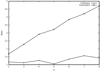
Finally, for inconsistent problems (dashed line), ratio is more important than for consistent ones. It increases with the number of solvers. In other words, obtained results for these problems are mostly due to cooperation and the contribution of cooperation increases with the number of solvers.
For inconsistent problems, we must underline the predominant role of values heuristics. For each solver ➳ (except one if the number of solvers is odd), there exists a solver which uses the same variables heuristic as ➳ and the values heuristic which is reverse with report to one of ➳ . Without exchanging nogoods, these two solvers visit similar search trees. With exchanging nogoods, each one explores only a part of its search tree thanks to received nogoods. It's the same for consistent problems, but this effect is less important because the search stops as soon as a solution is found.
We focus then on possible reasons of efficiency's decrease. With a scheme like our, an usual reason of efficiency's lack is the importance of cost of communications. Our method doesn't make exception. But, in our case, there is another reason which explains the decrease of performances.
We compare multiple solvers ➵ ➸ and ➵ ❩ ➸ . Both have 8 solvers. For ordering values, half solvers of ➵ ➸ use the appearance order, other half the reverse order. All solvers of ➵ ❩ ➸ use the appearance ➺ order. We realise that ➵ ➸ has a better efficiency than ➵ ❩ ➸ . The number of messages for ➵ ❩ ➸ is greater than for ➵ ➸ . But, above all, it's the same for the number of nodes. So ➵ ❩ ➸ explores more important trees. ➵ ➸ and ➵ ❩ ➸ differ in used heuristics for ordering values and variables. The heuristics we use for ordering variables are near each other. Using two different orders of values adds diversity to resolution. Thus, ➵ ➸ is more various than ➵ ❩ ➸ . This difference of diversity permits to explain the gap of efficiency between ➵ ➸ and ➵ ❩ ➸ . The lack of diversity is the main reason (with the increase of number of communications) of the efficiency's decrease.
Number of messages and real contribution of manager
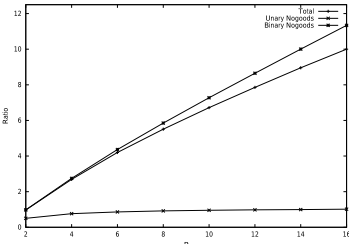
In order to measure the real contribution of manager, we compare the costs of communications in a scheme with manager and one without manager. In presented results, we consider that the cost of a message is independent of presence or not of the manager, and that the communication of a binary nogood is twice as expensive as one of a unary nogood (because a binary nogood consists of two pairs variable-value, against a single pair for a unary nogood). Figure 2 presents the ratio of cost of communications for a scheme without manager over one for a scheme with manager. Considered problems (consistent and inconsistent) belong to class (50,25,123,439). For information, we observe similar results for other classes.
P
Figure 2: Ratio between schemes with and without manager.
First, we note an increase of manager's contributionwith ② . Thus, we can hope that the number of solvers above of which the cost of communications penalizes efficiency is greater in a scheme with manager than one without manager.
More precisely, we note that communications of unary nogoods is more expensive in the scheme with manager, when ② is less important. This result was foreseeable. Indeed, in case of unary nogoods, the manager removes only doubles. As the probability that two solvers find simultaneously the same nogoods is all smaller since there are few solvers. We explain thus that the scheme with manager becomes better than one without manager when the number of solvers increases.
Regarding the cost of communications for binary nogoods, the scheme with manager is significantly cheaper and this economy increases with ② . This result is explained by the fact that binary nogoods are, in general, useful for few solvers. On overall communications, the scheme with manager is the best, due essentially to the number of binary nogoods which is significantly greater than one of unary nogoods (with a factor between 30 and 100).
In conclusion, the manager does its job by limiting the number of exchanged messages. It avoids solvers a lack of time due to management of messages (in particular, receipt of useless nogoods).
5 Conclusions and future works
In this paper, from an idea of Martinez and Verfaillie, we define a new scheme of cooperative parallel search by exchanging nogoods and we assess experimentally its efficiency. We observe then linear or superlinear speed-up up to 10 solvers for inconsistent problems and up to 16 solvers for consistent ones. So, exchange of nogoods is an efficient form of cooperation. We note a decrease of efficiency with the number of solvers, due to the increasing number of communications and to a lack of diversity of solvers.
A first extension of this work consists in finding several efficient and diverse heuristics in order to improve efficiency as well as increase the number of solvers. Then, we can extend our scheme by applying any algorithm which maintains some level of consistency, by using different algorithms (which would permit to combine complete search methods and incomplete ones like in [Hogg and Williams, 1993] and to improve the diversity of solvers), or by generalizing it to another form of cooperation with exchange of informations.
@inproceedings{ijcai2001p37,
  title     = {Cooperative Search and Nogood Recording},
  author    = {Terrioux, Cyril},
  booktitle = {Proceedings of the Seventeenth International Joint Conference on
               Artificial Intelligence, {IJCAI-01}},
  publisher = {International Joint Conferences on Artificial Intelligence},
  editor    = {Bernhard Nebel},
  pages     = {260--264},
  year      = {2001},
  url       = {https://ijcai.org/proceedings/2001/37},
}
TY - CPAPER TI - Cooperative Search and Nogood Recording AU - Terrioux, Cyril T2 - Proceedings of the Seventeenth International Joint Conference on Artificial Intelligence, IJCAI-01 PB - International Joint Conferences on Artificial Intelligence PY - 2001 SP - 260 EP - 264 UR - https://ijcai.org/proceedings/2001/37 ER -Copied
Machine-readable versions of this paper, for tools and AI agents:





