
Bounding the Suboptimality of Reusing Subproblem
Proceedings of the Sixteenth International Joint Conference on Artificial Intelligence. Uncertainty and Probabilistic Reasoning. Pages 1340-1346.
© 1999 International Joint Conferences on Artificial Intelligence
Abstract
We are interested in the problem of determining a course of action to achieve a desired objective in a non-deterministic environment. Markov decision processes (MDPs) provide a framework for representing this action selection problem, and there are a number of algorithms that learn optimal policies within this formulation . This framework has also been used to study state space abstraction, problem decomposition, and policy reuse. These techniques sacrifice optimality of their solution for improved learning speed. In this paper we examine the suboptimality of reusing policies that are solutions to subproblems. This is done within a restricted class of MDPs, namely those where non-zero reward is received only upon reaching a goal state. We introduce the definition of a subproblem within this class and provide motivation for how reuse of subproblem solutions can speed up learning. The contribution of this paper is the derivation of a tight bound on the Joss in optimality from this reuse. We examine a bound that is based on Bellman error, which applies to all MDPs, but is not tight enough to be useful. We contribute our own theoretical result that gives an empirically tight bound on this suboptimality.
- [Bertsekas, 1987] D.P. Bertsekas. Dynamic Programming: Deterministic and Stochastic Models. Prentice-Hall, En- glewood Cliffs, NJ, 1987.
- [Dean and Lin, 1995] T. Dean and S.-H. Lin. Decomposition techniques for planning in stochastic domains. In Proceed- ings of the Fourteenth International Joint Conference on Artificial Intelligence (JJCAJ-95), 1995. IJCAI
- [Hauskrecht et al., 1998] M. Hauskrecht, N. Meuleau, L. P. Kaelbling, T. Dean, and C. Boutilier. Hierarchical solu- tion of markove decision processes using macro-actions. In Proceedings of the Fourteenth Annual Conference on Uncertainty in Artificial Intelligence (UAJ-98), 1998.
- [Kaelbling et al., 1996] L. P. Kaelbling, M. L. Littman, and A. W. Moore. Reinforcement learning: A survey. Journal of Artificial Intelligence Research, 4:237-285, 1996.
- [Parr, 1998] R. Parr. Flexible decomposition algorithms for weakly coupled markov decision problems. In Proceed- ings of the Fourteenth Annual Conference on Uncertainty in Artificial Intelligence ( UAJ-98), 1998.
- [Sutton et al., 1998] R. Sutton, D. Precup, and S. Singh. Be- tween MDPs and semi-MDPs: Learning, planning, and representing knowledge at multiple temporal scales. Tech- nical report, Department of Computer Science, University of Massachusets, Amherst, 1998.
- [Thrun and Schwartz, 1995] S. Thrun and A. Schwartz. Finding structure in reinforcement learning. In G. Tesauro, D. Touretzky, and T. Leen, editors, Advances in Neural In- formation Processing Systems, volume 7, pages 385-392. The MIT Press, 1995.
- [Veloso, 1994] M. M. Veloso. Flexible strategy learning: Analogical replay of problem solving episodes. In Pro- ceedings of AAAI-94, the Twelfth National Conference on Artificial Intelligence, pages 595-600, Seattle, WA, Au- gust 1994. AAAI Press.
- [Watkins, 1989] Christopher J. C. H. Watkins. Learning from Delayed Rewards. PhD thesis, King's College, Cam- bridge, UK, 1989.
- [Williams and Baird, 1993] R. J. Williams and L. C. Baird. Tight performance bounds on greedy policies based on im- perfect value functions. Technical report, College of Com- puter Science, Northeastern University, 1993.
References were extracted automatically from the PDF and may contain errors.
Full text extracted automatically from the PDF; figures, tables and equations may differ. The PDF is the version of record.
1 Introduction
Selecting a course of action in a complex environment is a difficult task. It has been examined in a number of frame works, including classical planning, probabilistic planning, and Markov decision processes. In all of these formula tions it is a goal to solve difficult problems through simpli fying techniques, such as finding and exploiting levels of state abstraction [Hauskrecht et al., 1998; Parr, 1998], de composing into smaller subproblems [Dean and Lin, 1995], and reusing previously discovered solutions [Veloso, 1994; Thrun and Schwartz, 1995]. All of these techniques make lo cally optimal "decisions" and therefore will almost certainly find a suboptimal solution. The tradeoff is to sacrifice opti mality of the solution for efficiency in finding it.
In this paper we examine this tradeoff in the context of Markov decision processes (MDPs). We assume the reader has a basic understanding of MDPs [Kaelbling et al., 1996], though we will give a brief overview emphasizing the theory that is needed for this paper. We will formalize a notion of a subproblem and what it means to use a subproblem. We will then provide examples of the use of subproblem solutions, and also the tradeoff between suboptimality and efficiency. The focus of the paper is the introduction of a quantitative bound on this loss of optimality. We will examine a bound based on Bellman error, which does not give us a tight bound. We contribute our own theoretical result and show empirical results that this bound is tight using our presented examples.
2 Markov Decision Processes
A Markov Decision Process, Pis a tuple (S, A , T , R), where S is a set of states, A is a set of actions, T is a transition functionS x A x S -+ [0 , 1], and R is a reward function S x A -+ R. The transition function defines a probability distribution over next states as a function of the current state and the agent's action. The reward function defines the re ward received when selecting an action from the given state. The goal is to find a policy, 1r : S -+ A, which determines the agent's actions so as to maximize discounted future reward, with discount factor I·
For any policy, 1r, the value of a state, V,., is the expected discounted future reward of following the policy 1r from that state. We say 1r* is the optimal policy and V* is the value function of the optimal policy. A standard result from the theory of dynamic programming [Bertsekas, 1987] states that the optimal value function is the unique solution to the simul taneous equations for all states, s,
These equations are called the Bellman equations. For any value function, V, not necessarily optimal, we can define the Bellman residual or Bellman error as,
So the optimal value function has a Bellman error of 0, and reinforcement learning techniques, in general, can be viewed as trying to minimize the Bellman error.
In this paper we will examine a restricted class of MDPs, called goal state MDPs. MDPs in this class have a set of goal states. Reaching a goal state ends the trial, so all actions from a goal state simply transition to the same state with zero reward. Other transitions into goal states receive a reward of 1, and all other transitions receive a reward of 0. Using this class we can replace the reward function R with the goal set G ~ S since this uniquely defines the reward function. Throughout this paper we will refer to MDPs in this class as the tuple (S, A, T, G).
3 Subproblems
Before we can proceed we need to formalize the notion of a subproblem within the frameworks of our restricted class of MDPs. We also need to define what it means to use a subprob lem. These notions hinge on the definition of the boundary of a set of states.
Definition 1 For a set of states, S, let the boundary of S, denoted B(S), be the set of all states not inS with a non-zero probability transition from a state inS.
In other words the boundary of S are all the states not in S that are reachable from S in a single time step.
We can now define our notion of a subproblem.
Definition 2 A subproblem, S, of an MDP, P (S, A, T, G), is a pair (S' , G') satisfying:
- S;,G' ~ S,
- S' n G = 0 and B(S') n G = 0,
- G' ~ B(S').
This definition induces a new MDP over the states S'. The state transitions remain the same as in P, but the reward func tion is zero for all transitions except those entering states in G', where the reward is one.
Given this notion of a subproblem we want to investigate the effects of using a subproblem solution. So we define a formal notion of using a subproblem.
Definition 3 For a subproblem, S = (S', G'), of a problem P, we say that a policy, 1rjor P uses S if and only if 1r re stricted to states in S' is optimal for the subproblem, S. Ad ditionally, the optimal policy for P that uses Sis denoted 1r.$.
4 Examples
Given this definition of subproblems and how they are used, we want to examine the tradeoffs of reusing subproblem solu tions. We explored this in the context of some simple stochas tic maze problems, which are within our class of goal state MDPs. The two problems discussed here are representative of more complex MDPs.
4.1 Hallway Example
Figure 1 depicts a simple grid environment that was first in vestigated by Thrun and Schwartz [1995] within the context of sharing policies. The agent has actions that move it in any of the eight grid directions (including diagonal moves), but with probability 0.1 its action is ignored and it is moved in a random grid direction. There is a single goal state labeled 'G' in the diagram. The agent receives a reward of 1 for a tran sition into the goal state, and a reward of 0 otherwise. The agent is trying to maximize its discounted future reward with a discount factor, 1 = 0.9.
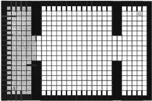
The shaded regions in the diagram denote subproblems. For example the subproblem of exiting the left room has the dark shaded region as its state space, S'. The five states in the rightmost half of the doorway into the middle room are the boundary of S', and in this case G' = B(S'). Another subproblem is exiting both the left and middle rooms. In this case the states, S', would be both shaded regions, and the goal states would be the five rightmost states of the doorway to the room on the right.
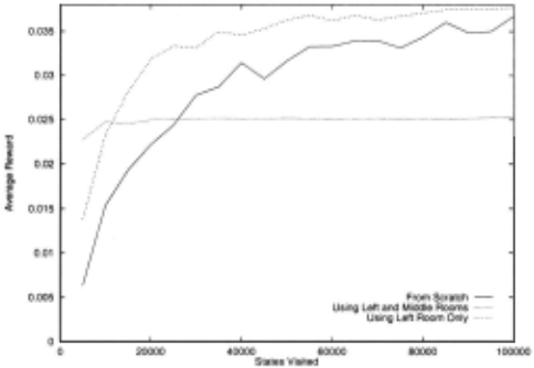
We explored how using the solution to these subproblems might speed learning of the complete problem. We fixed the policy to always select the subproblem's optimal action while within the subproblem's state space (i.e. the shaded regions.) We then use Q-Learning [Watkins, 1989] with a decreasing learning factor in order to learn the optimal policy given this constraint.
The results of this Iearni1_1g can be seen in figure 2. When we use the subproblem of exiting the left and middle rooms, we have a huge boost in learning speed. After visiting 5000 states, it performs approximately six times better than learn ing from scratch. Notice that this sacrifices convergence to the optimal solution. The more conservative approach of using the subproblem of exiting just the left room has a more conservative learning improvement. After visiting 5000 states it performs almost three times better than learning from scratch. Although the improvement isn't as pronounced, it appears to converge to an optimal solution.
4.2 Doorways Example
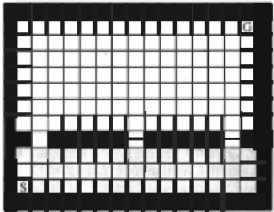
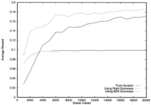
A second example that we explored consisted of a similar grid world but with multiple doorways, where G' =F B(S'). This is depicted in figure 3. The actions and transitions remain the same as was described for the hallways example. Like that example, this also has intuitive subproblems, such as reach ing a subset of the three doorways. We explored this domain using a number of these subproblems. Results are shown in figure 4 for learning when using the subproblem of reaching the right doorway, reaching either the right or middle door way, and learning from scratch.
The results are very similar to the previous example. Sub problems speed learning but are likely to converge on a sub optimal solution. These results also motivate our goal, to be able to make a claim about the amount of optimality sacri ficed in order to gain the improved learning speed.
5 Bounding the Suboptimality
In order to better judge this tradeoff it is important to know the suboptimality of the solution obtained. Formally, we want to find a bound on the suboptimality of 1r:;. This would pro vide us with a quantitative measure of the trade-off of using S as a subproblem. Before we discuss possible bounds we need a notion of suboptimality.
Definition 4 A policy, 1r, is a-optimal if and only if Vs V" (s) 2: aV*(s).
Using this definition, a values are in the range (0 , 1], where large values are closer to the optimal solution. A summary of the optimality for our examples (figures 2 and 4) is given in table 1, under the column labeled "actual". These values were computed by taking the minimum over all states of the ratio between the value of the state when using the subproblem and the optimal value of the state. We can quantify our goal as finding a guaranteed lower bound for these values without requiring knowledge of the optimal policy or value.
We will first examine a bound based on Bellman error and give some empirical results on our examples that show that this bound is not satisfactorily tight. We will then introduce a new bound based on boundary values and show its results on these same examples.
5.1 Bound Using Bellman Error
The use of the Bellman error to bound the suboptimality of a policy was developed by Williams and Baird [1993]. Bellman error, as mentioned earlier, is simply the maximum error in the Bellman equations, and the optimal policy would have a Bellman error of zero. They proved the following for all MDPs,
Theorem 1 For any value function, V, with Bellman error, c. Let 1r be a policy greedy for V. Then for all states, x,
Qualitatively, this means we can bound the suboptimality of a policy by examining the Bellman error of a value function that induces that policy.
We can use this to compute a bound by simply calculating the Bellman error of V$. We define a value function that in duces 1r5 and satisfies the Bellman equations for states in S (because we are using an optimal solution to the subproblem) and also for states outside of S (because we are acting op timally outside of S.) Then the only states with a non-zero Bellman error would be on the boundary of S.
Results from the Examples. Table 1 gives the results of using this bound in the subproblems in section 4. These val ues were computed by finding the optimal solution using the subproblem, calculating the Bellman error for that value func tion, and applying the equation. The results are quite disap pointing. Even for subproblems that are nearly optimal (e.g. the left and middle rooms of the hallway problem) result in a weak constraint on the suboptimality. The computed bound does not help identify when a subproblem results in a good solution.
| Optimality | ||||
|---|---|---|---|---|
| Example | Subproblem | Actual | Bellman Bound | Boundary Bound |
| Hallway | Left and Middle Rooms | 0.66 | 0.01 | 0.65 |
| Left Room | 0.99 | 0.22 | 0.98 | |
| Doorways | Right and Middle Doorway | 0.99 | 0.38 | 0.77 |
| Right Doorway | 0.52 | 0.04 | 0.16 | |
5.2 Bound Using Boundary Values
The following two definitions play a crucial role in our bound on suboptimality. The first provides a quantitative measure of the stochasticity of a problem. The second provides a mea sure for comparing values of sets of states.
Definition 5 Let Ps be the probability that following the op timal policy at s will transition to a state, s'' where v· ( s') < v· (s). Let p = maxs ES Ps· This captures the stochasticity of the problem, where p = 0 for a deterministic problem.
Definition 6 For a set of states 51 and 52, and a policy 1r, we say 51 2: ~ 52 if and only if,
If 5 2:~ 5 then 5 is a -equivalent with respect to 1r, i.e. the values of all the states in the set are within a.
The following theorem provides a bound on the subopti mality of using a subproblem where the goal states for the subproblem are its entire boundary.
Theorem 2 Given a subproblem S (5' , B(5')) of P , if B(5') is a -equivalent with respect to 7rs, then, 7rs is af3-optimalforP,
The(]' value may appear cryptic but it is simply the discounted probability of ever reaching a state of lower value. The value emerges from the proof which is presented in appendix A.
We have attempted to generalize the theorem to all sub problems with the following conjecture,
Conjecture 1 Given a subproblem S = ( 5', G') of P, let G' = B(5')\G'. IfG' 2: ~~ G' and G' ::; ~~ 5, then 7rs is a 1a2f3-optimalforP,
Theorem 3 Conjecture I is true ifP is deterministic (i.e. if p = 0.)
Theorem 3 proves the conjecture true for deterministic MDPs and the f3 factor should provide the necessary adjust ment for the non-determinism as it did in theorem 2. The proof for theorem 3 is given in appendix B.
Results from the Examples. Table 1 gives the results of using this bound in our example subproblems. The values were computed much like those for the Bellman error; an op timal solution was learned using the subproblem, the a values were calculated, and the bound computed. The results show a reasonably tight bound, especially for the single exit sub problems. Thought it's not as tight on the multiple exit sub problems it is still much improved over the bound computed from Bellman error.
This bound provides considerable information as to the loss in optimality of using a subproblem. In addition to this guarantee on the resulting policy it also helps to identify a possibly better subproblem. This is done by examining the a values. For example, in the doorways problem using the right doorway, the guaranteed optimality is fairly weak. But, by examining the a values it becomes obvious that this bound could be improved if the middle door was in the subproblem's goal states. By using the "new" subproblem we achieve a bet ter policy and a better bound on its suboptimality.
6 Related Work
The definitive performance bound for general MDPs is the one based on Bellman error [Williams and Baird, 1993]. It is provably tight for the general case of any value function of any MDP. Although, as seen earlier, it is not as strong at bounding subproblem use in our restricted class of MDPs.
There has been a great deal of recent work in finding and exploiting layers of abstraction in MDPs. This work is very related to subproblem reuse since we can view the operators of a high layer of abstraction as subproblem solutions of the lower layers. Therefore, theoretical bounds on the subopti mality of subproblem reuse can also help to understand the suboptimality of using abstractions.
Sutton and his colleagues provided a theoretical frame work for dealing with abstraction in reinforcement learning, through a multi-time model [Sutton et al., 1998] . This frame work defines temporally abstract options or macro-actions, which are local policies that act like subroutines. Options, unlike primitive actions, can control the agent over multiple time steps, and so can work at different levels of abstraction . The theoretical model of options allows them to be treated as actions in the MDP, and can be used to possibly speed plan ning and still find an optimal solution.
Hauskrecht, eta!. [1998] extend Sutton's original theoret ical results on planning with macro-actions to develop a hi erarchical model of MDPs that reduces the size of the state and action space. This is done by creating a state partition of the MDP and restricting a macro to be a local policy over one of these regions. This partition and associated macros defines a new abstract MDP whose states are the boundaries of the regions, and whose actions are the macros that move between regions. The optimal solution to this abstract MDP can then be used as a solution to the original MDP.
To make some guarantees on the quality of such a solution, a macro set is required that "covers" the range of values of a region's exit states. Such a macro set limits the resulting Bellman error and makes use of the Bellman bound to guar antee some amount of optimality. Unfortunately, construction of such a macro set will often be intractable. The number of required macros grows exponentially in the number of exit states for the region and in the desired bound on suboptimal ity.
Parr [1998] developed a number of improved methods for constructing macro sets, or policy caches, for an abstract MDP. He presents two algorithms that give optimality guaran tees on the original MDP, which are not exponential in neither the error bound nor the size of the region's boundary. These techniques still use the Bellman bound as the measure of sub optimality, and still can create a much larger macro set than is actually required.
7 Conclusion
In this paper we examined the reuse of subproblem solutions in the context of goal state MDPs. We gave a formal defi nition for a subproblem, and what it means to use subprob lems in this context. We also provided representative ex amples of the tradeoff between learning speed and loss in optimality when reusing subproblems. In order to quantify this tradeoff we examined quantitative bounds on the subop timality of these techniques. Although generally applicable, a bound based on the Bellman error is often not tight enough to be useful. We contributed the derivation of an empirically tight bound that applies specifically to subproblems in our re stricted class of MDPs.
This work opens further directions to investigate, includ ing relaxing the restriction on the applicable class of MDPs, examining the effects of using multiple subproblems, and in vestigating if our bound may help to retrieve the most useful subproblems.
A Proof of Theorem 2
Proof. The proof makes use of a special non-stationary pol icy, 1r. This policy initially selects the same action as 1r5 for states in S', and the same action as 1r* for states not in S'. After reaching a state in B ( S') the policy changes so that it always selects the same action as 1Ts. Notice that v.; ( s) 2: V,. ( s) V s E S . This is because 1r uses S, and non-stationary policies cannot do better than an optimal sta tionary one.
Letsm = argmax·EB(S')V*(s). Wewillfirstshowthat1r.S is ,8-optimal for sm. From this we will be able to show that for all other states it is a ,B-optimal.
We can write v· ( Sm) as,
We can then split the sum into the paths containing a state in S' and those that don't contain a state in S'. Let p be the probability a path from sm, following the optimal policy, contains a state in S'. Then, ·
Let II= (1- p)E(Value(path)IS' npath = 0). Notice that any path that contains a state in S' must also contain a state in B(S'). So we can write the second term as a value of that state discounted by the length of the path before the .state is reached. Let f(path , s) be the number of steps in path until s is reached. So,
Since v· ( Sm) 2: v· ( s)' we can substitute v· ( Sm) for v· ( s) and pull it outside of the sum. The resulting sum is just the expected discount between sm and s when following the op timal policy. Let this value be o. So we get,
We can also achieve a similar result for VS' ( sm). Since our non-stationary policy, 1r, acts the same as 1r· for s rt S', then it will achieve the same value for paths not containing s E S'. As before, paths containing a state in S', must contain a state in B ( S'). And upon entering this state 1r will select actions according to 1Ts. So we can write,
By the a-equivalence of B(S') we know that v;(s) 2: a VJ ( sm). So we can substitute a VJ ( sm) for VS' ( s) and pull it outside of the sum. The resulting sum is the expected dis count between sm and s when following 1!" . Let this value be o'. So we get,
Since 1r is optimal over the subproblem, it will reach a state in B(S') with no worse expected discount than 1r*. Hence, o' 2: o, and we can substitute o foro' and maintain the inequality.
Now we examine the ratio of the two values,
The value, po, is the probability of returning to a state in S', discounted by the distance to that state and the distance from that state to a state in B(S'). Since all states in S' have a smaller value than sm, we can bound this by the discounted probability of ever reaching a state with smaller value, which can be computed from p,
So, po ::; (j, hence,
We can now show that 1r.5 is o:/3-optimal for any state, s. We can decompose the value of s just as was done for sm. Let p be the probability that a path from s, following 1r*, contains a state in S'. Notice that if s E S', then p = 1.0. We let v and r5 represent the same values with respect to s. Then we can bound V*(s), VS'(s), and their ratio as follows:
Hence 1r$ is o:f3-optirnal for P.
B Proof of Theorem 3
Proof. Since P is deterministic then p = 0 and f3 = 1. Also, for any state, s, and a policy there is a unique path of states to a state in G that follows that policy. Trivially, if the optimal path (path of states from following the optimal policy) from s does not contain a state in S' then v; ( s) = V* (s). ·
Consider the case where the optimal path from s contains a state inS'. Then it must contain a state in B(S'). Let g be the last state in the optimal path where g E B(S'). So the optimal path from g cannot contain a state in S', and therefore,
Now, there are two cases:
- g E G'. The path from following 1r5 will reach a state g' E G' in fewer steps (because 1r.5 is optimal at reaching goal states of the subproblem.) Since G' 2:~~ G', then
and since g' is reached in fewer steps,
0
@inproceedings{ijcai1999p190,
  title     = {Bounding the Suboptimality of Reusing Subproblem},
  author    = {Bowling, Michael H. and Veloso, Manuela M.},
  booktitle = {Proceedings of the Sixteenth International Joint Conference on
               Artificial Intelligence, {IJCAI-99}},
  publisher = {International Joint Conferences on Artificial Intelligence},
  editor    = {Thomas Dean},
  pages     = {1340--1346},
  year      = {1999},
  note      = {Uncertainty and Probabilistic Reasoning},
  url       = {https://ijcai.org/proceedings/1999/190},
}
TY - CPAPER TI - Bounding the Suboptimality of Reusing Subproblem AU - Bowling, Michael H. AU - Veloso, Manuela M. T2 - Proceedings of the Sixteenth International Joint Conference on Artificial Intelligence, IJCAI-99 PB - International Joint Conferences on Artificial Intelligence PY - 1999 SP - 1340 EP - 1346 UR - https://ijcai.org/proceedings/1999/190 ER -Copied
Machine-readable versions of this paper, for tools and AI agents:





