
Computing Factored Value Functions for Policies in Structured MDPs
Proceedings of the Sixteenth International Joint Conference on Artificial Intelligence. Uncertainty and Probabilistic Reasoning. Pages 1332-1338.
© 1999 International Joint Conferences on Artificial Intelligence
Abstract
Many large Markov decision processes (MDPs) can be represented compactly using a structured representation such as a dynamic Bayesian network. Unfortunately, the compact representation does not help standard MDP algorithms, because the value function for the MDP does not retain the structure of the process description. We argue that in many such MDPs, structure is approximately retained. That is , the value functions are nearly additive: closely approximated by a linear function over factors associated with small subsets of problem features. Based on this idea, we present a convergent, approximate value determination algorithm for structured MDPs. The algorithm maintains an additive value function, alternating dynamic programming steps with steps that project the result back into the restricted space of additive functions. We show that both the dynamic programming and the projection steps can be computed efficiently, despite the fact that the number of states is exponential in the number of state variables.
- [Bacchus and Grove, 1995] F. Bacchus and A. Grove. Graphical models for preference and utility. In Proc. UAI, 1995.
- [Boutilier and Dearden, 1996] C. Boutilier and R. Dearden. Ap- proximating value trees in structured dynamic programming. In Proc. ICML, pages 54-62, 1996.
- [Boutilier et al., 1998] C. Boutilier, R.I. Brafman, and C. Geib. Pri- oritized goal decomposition of Markov decision processes: To- wards a synthesis of classical and decision theoretic planning. In Proc. UAI, pages 24-32, 1998.
- [Boutilier et al., 1999] C. Boutilier, T. Dean, and S. Hanks. De- cision theoretic planning: Structural assumptions and computa- tional leverage. Journal of Artificial Intelligence Research, 1999.
- [Boyen and Koller, 1998] X. Boyen and D. Koller. Tractable infer- ence for complex stochastic processes. In Proc. UAI, 1998.
- [Dean et al. , 1997] T. Dean, R. Givan, and S. Leach. Model reduc- tion techniques for computing approximately optimal solutions for Markov decision processes. In Proc. UAI, 1997.
- [Gordon, 1995] G.J. Gordon. Stable function approximation indy- namic programming. In Proc. ICML, pages 261-268, 1995.
- [Howard and Matheson, 1984] R.A. Howard and J.E. Matheson. Influence diagrams. In Readings on the Principles and Applica- tions of Decision Analysis, pages 721-762. Strategic Decisions Group, 1984.
- [Keeney and Raiffa, 1976] R.L. Keeney and H. Raiffa. Decisions with Multiple Objectives: Preferences and Value Tradeoffs. Wi- ley, 1976.
- [Meuleau et al., 1998] N. Meuleau, M. Hauskrecht, K-E. Kim, L. Peshkin, L.P. Kaelbling, T. Dean, and C. Boutilier. Solving very large weakly coupled Markov decision processes. In Proc. AAAI, pages 165-172, 1998.
- [Nelson, 1958] E. Nelson. The adjoint Markoff process. Duke Mathematical Journal, 25, 1958.
- [Singh and Cohn, 1998] S.P. Singh and D. Cohn. How to dynami- cally merge Markov decision processes. In NIPS 10, pages 1057- 1063, 1998.
- [Strang, 1980] G. Strang. Linear Algebra and Its Applications. Academic Press, 1980.
- [Sutton et al., 1999] R.S. Sutton, S. Singh, D. Precup, and B. Ravindran. Improved switching among temporally abstract actions. In NIPS 12, 1999. To appear.
- [Tadepalli and Ok, 1996] P. Tadepalli and D. Ok. Scaling up aver- age reward reinforcement learning by approximating the domain models and the value function. In Proc. ICML, 1996.
- [Tsitsiklis and Van Roy, 1996] J. D. Tsitsiklis and B. Van Roy. Feature-based methods for large scale dynamic programming. Machine Learning, 22( 1):59-94, January 1996.
- [Van Roy, 1998] B. Van Roy. Learning and Value Function Ap- proximation in Complex Decision Problems. PhD thesis, Mas- sachusetts Institute of Technology, 1998.
References were extracted automatically from the PDF and may contain errors.
Full text extracted automatically from the PDF; figures, tables and equations may differ. The PDF is the version of record.
1 Introduction
Over the past few years, there has been a growing interest in the problem of planning under uncertainty. Markov decision processes (MDPs) have received much attention as a basic semantics for this problem. An MDP represents the domain via a set of states, with actions inducing stochastic transitions from one state to another. The key problem with this type of representation is that, in virtually any real-life domain, the state space is quite large. However, many large MDPs have significant internal structure, and can be modeled very com pactly if that structure is exploited by the representation. In factored MDPs, a state is described implicitly as an assign ment of values to some set of state variables. A dynamic Bayesian network can then allow a compact representation of the transition model by exploiting the fact that the transi tion of a variable usually depends only on a small number of other variables. In a simple robotics example, the location of the robot at time t + 1 may depend on its position, velocity, and orientation at time t, but not on what it is carrying. The momentary rewards can often also be decomposed: as a sum
Ronald Parr
Computer Science Department Stanford University parr@cs.stanford.edu
of rewards related to individual variables or small clusters of variables. In our robot example, our reward might be a sum of two subrewards: one associated with location (for getting too close to a wall) and one associated with the printer status (for letting paper run out).
While these representations allow very large, complex MDPs to be represented compactly, they do not help address the planning problem. Standard algorithms for solving MDPs require the representation and manipulation of value func tions - functions from states to values. Since a state is a full instantiation of all state variables, the representation of the full value function is exponential in the number of state variables. Unfortunately, structure in a factored MDP does not, in general, guarantee any type of structure in the value function. Even some very simple MDPs with very compact transition models and fully decomposed rewards lead to value functions that have no usable structure whatsoever (see Sec tion 2). Thus, algorithms that represent the value function exactly will be impractical for dealing with many large, struc tured domains.
One approach to controlling the size of the value function representation is to use a truncated value function that ignores some state variables. Several methods exist for detecting ir relevant state variables. A closely related approach uses ap proximate or abstract model that eliminates some state vari ables. (See Boutilier et al. [1999] for a survey of these ap proaches.) These methods have the common limitation that they can force different states to have the same value, pro ducing a coarse-grained approximation to the value function with large plateaus of indistinguishable states.
Our work is based on the intuition that, while value func tions might not be structured, there are many domains where they are · ~close" to having exploitable additive structure. Con sider, for example, a stochastic version of a traditional plan ning task, where several subgoals can contribute to the over all success of the plan. Here, it is quite plausible that the value of a state is approximately linear in the set of subgoals achieved at that state (with more important subgoals having, perhaps, a higher weight). Clearly, this is only an approxi mation, as subgoals might interact in various ways; however, it may be a fairly good approximation. Furthermore, if some subgoals interact strongly, we can have value function com ponents that depend on the status of several subgoals. Such value functions have a long history in multi-attribute utility theory [Keeney and Raiffa, 1976]; they also play a central role in influence diagrams [Howard and Matheson, 1984].
Based on this intuition, we propose a new approach to com puting approximate value functions for structured MDPs. We restrict attention to value functions that are a linear combi nation of local basis functions, each of which depends only on a small subset of the state variables. As discussed above, we believe that, in many cases, such a value function can be a good approximation to the correct value function. In par ticular, unlike the coarse-grained approximations discussed above, this approximation can as.sign a distinct value to every state. However, it can still be represented compactly using a small number of parameters (the coefficients of the basis functions) . We propose to use algorithms whose entire com putation is restricted to value functions that are compactly represented in this form.
Our focus in this paper will be on the value determination task: computing the value function associated with a particu lar policy. This task can be solved using a simple algorithm that iterates through a dynamic programming step, gradually converging to the correct value function. Our algorithm aug ments this basic iteration with an additional projection step, where the value function resulting from each dynamic pro gramming step is projected back down into the "allowable" space of value functions.
There are several key issues that arise in such an algorithm. First, we must show how the operations required by such an algorithm- dynamic programming and projection- can be executed efficiently. One of our main contributions is that we provide, for both of these steps, an efficient algorithm that de pends upon the size and structure of the model and basis func tion representations, not upon the exponentially sized state space. We note that we can accomplish these operations ef ficiently despite the fact that each of the exponentially many states may have a distinct value. Second, we must show that the algorithm behaves reasonably: that it converges to a sta ble fixed point, hopefully one which is close to the true value function . By a careful choice of distance metric, we can show conditions under which the algorithm will converge to a solu tion which is not too far away from the best value function de scribable in the restricted space. Finally, we must show how to apply this algorithm to the task of evaluating policies in a factored MDP. This application is far from trivial, as policies in a large MDP may be very complex. We show that our al gorithm allows effective policy evaluation for policies repre sented as a small set of conjunctive decision rules (e.g., deci sion trees); this class is arguably the most widely used class of compactly represented policies [Boutilier and Dearden, 1996; Dean et al., 1997].
2 Preliminaries
We begin by introducing some of the basic concepts that we will be using. Our primary focus is on the value determination problem. Thus, for the time being, we will restrict attention to processes without a decision component. A Markov Process (MP) is defined as a triple (S, R , P) where: S is a set of states; R is a reward function R : S f-7 JR, such that R( s) represents the reward obtained by the agent in state s; P is a transition model, so that P( s' I s) represents the probability of going from state s to state s'.
A Markov process is associated with a value function V : S f-7 JR, where V(s) is the total cumulative value that the agent gets if it starts at state s. We will be as suming that the MP has an infinite horizon and that future rewards are discounted exponentially with a discount fac tor r· Thus, V is defined using the fixed point equation V(s) = R(s)+r l::s' P(s' I s)V(s'). A simpleiterativepro cess can be used to perform value determination. We choose V 0 = 0. 1 We then repeatedly execute a dynamic program ming (DP) step:
We use T to denote the operator that takes a value function y (t) and returns y{t+l). We call y{t+l) the backprojection of y(t). Repeated applications ofT are known to converge to the true value function v·.
In a factored MP, the set of states is described via a set of random variables X = {X1, ... ,Xn}, where each Xi takes on values in some finite domain Val(Xi)· A state x defines a value Xi E Val(Xi) for each variable x i . The transition model is described as a dynamic Bayesian net work ( DBN). Let Xi denote the variable Xi at the current time and XI the variable at the next step. The transition graph is a two-layer directed acyclic graph whose nodes are {X1, . .. , Xn, X{, . .. , X~}. In this paper, we will as sume that all edges in this graph are directed from nodes in {X1 , . .. ,Xn} to nodes in {X{, ... , X~}. (This assumption can be relaxed, but the resulting algorithm becomes some what more complex. We defer details to a longer paper.) We denote the parents of X I in the graph by Pa(XI) . Each node XI is associated with a conditional probability table (CPT) P(XI I Pa(XD). The transition probability P(x' I x) is then defined to be fL P(x~ I u i), where u i is the value in x of the variables in Pa(XI).
We also need to provide a compact representation of the reward function . As discussed in the introduction, we assume that the reward function is factored additively into a set of localized reward functions, each of which only depends on a small set of variables. In general, we say that a function f is restricted to a set of variables C if f : Val( C) r-+ JR. Let R1, . . . , Rr be a set of functions , where each Ri is restricted to a cluster of variables Wi c {X1, . .. , Xn}, such that Ri : Val(Wi) r-+ JR. The reward function associated with the state xis then defined to be 2::~= 1 Ri(x) E JR. We note that, here and in the future, we use the following shorthand: iff is a function over some set of variables Y, and Y C Z, we will use f(z) to denote the value that f takes over the part of the vector z that corresponds to variables in Y.
One might be led to believe that factored transition dynam ics and rewards would result in a structured value function . Unfortunately, this usually is not the case. As we execute DP steps, the value function typically becomes more complex.
1 We begin with V 0 = 0 by convention. Any choice for V 0 will converge to the same fixed point.
Example 2.1: Assume that we have only a single reward function R that depends only on X 1 ; V(l) = R, so it also depends only on X 1 . Consider the summation in the DP step for V( 2 l:
where u is the instantiation of Pa(X{) in x. Thus, V( 2 ) de pends on X1 and on the entire parent set of X1 . Similarly, V( 3 ) depends on the union of all of their parents, etc. I
In general, the value function will eventually depend on all of the variables that have any influence whatsoever, direct or indirect, on a reward. In practice, this set will typically be all of the state variables, as it is somewhat superfluous to intro duce into the process description variables whose value never matters to the agent's utility.
3 Constrained value determination
As we described in the introduction, the key idea behind our approach is the restriction of our algorithms to the use of value functions in a limited class. This idea is best known under the name value function approximation, which is used frequently in the context or reinforcement learning [Tade palli and Ok, 1996; Van Roy, 1998]. We use this idea in the context of maintaining full value functions and propa gating them through the DP equation (l) [Gordon, 1995; Tsitsiklis and Van Roy, 1996]. However, unlike other meth ods, which deal with large state spaces by considering only a restricted set of "representative" states, our method efficiently finds a least squares approximation for the entire state space.
More precisely, let V ~ IRs be a restricted set of value functions. We will define V via a set of basis functions H = { h1 , ... , hm}. That is, we have that H is a basis for V[H] ~ IR 5 if every function V E V(H] can be written as V = 2::}: 1 Wj hi for some weights w1 , ... , Wj.
Our algorithm repeatedly executes the following steps. It begins with a value function lf(t) E V. It then backprojects it via (1), resulting in a value function y(t+l). In general, the DP step does not maintain the property of being in a restricted class V. Therefore, we typically have that y(tH) f/. V. We then project y(t+ 1 ) into V, i.e., find the "closest" value func tion in V. The result is our new value function lf(tH).
We must decide what it means for a value function V E V to be "close" to some other value function V by choosing a suitable distance measure. Several constraints combine to make this choice difficult. On the one hand, we need a con traction property: exact value determination converges be cause (I) is a contraction- each iteration decreases the error of V(t) by a constant factor. In order to get convergence for approximate value determination, we need a similar contrac tion properti We also need an effective algorithm for pro jecting into V, relative to this distance. Finally, we need this projection operation to be a non-expansion under the same distance, otherwise we are not guaranteed the desired conver gence property. Tsitsiklis and Van Roy [ 1996] underscore the importance of this point by demonstrating a two-state MDP for which this type of approximate value determination di verges if we use standard least-squares approximation. Un fortunately, it turns out to be nontrivial to find a distance met ric that satisfies all criteria. For example, (1) is not a con traction in Euclidean distance. It is a contraction in L 00 and £ 1 norms 2 , but we have no efficient projection algorithm for these distances.
One choice that turns out to satisfy both desiderata is the weighted Euclidean distance. Let p(s) be the occupancy probability of the state s in the stationary (steady-state) dis tribution p. 3 We define the weighted Euclidean distance dp(V, V) as Ls p(s)(V(s) - V(s)) 2 . We say that V is the least dp projection of V into V if V E V is the function in V that is closest to V in terms of dp. Intuitively, unweighted Euclidean distance places equal emphasis on getting each V(s) as close as possible to V(s), whereas the weighted distance places more emphasis on getting correct values for states that are visited more often.
Fortunately, there exists a fairly straightforward algorithm for doing projection relative to weighted Euclidean distance. The key operation is the weighted dot product. For two func tions J,g E IRs, we define(! · g)p = Ls p(s)f(s)g(s). We define the length lp(hj) = (hj · hj )p. To project a function V into V[H], we first compute each coefficient wj = (hi · V)p/lp(hj). This intermediate weight vector w' = ( w~, . .. , w~) t has to be transformed, in order to ac commodate for any (linear) dependencies between our basis vectors. We define aij = (hi · hj )p. and define A to be the matrix ( aij). If we now define a weight vector w = A - 1 w', we know that 2::}: 1 Wjhj is the least dp projection of V into V [Strang, 1980]. We define Pp to be the operator that projects into V.
The contraction of the T operator in dp distance is estab lished in Nelson [1958] and is combined with projection in Van Roy [ 1998], yielding:
Theorem 3.1: (a) The operator T is a contraction in dp dis tance with rate "( < 1; hence, T has a unique fixed point V*. (b) LetT = Pp T Then Tis a contraction in dp dis tance with rate"' ::; "(;hence, t has a unique fixed point v·. Furthermore, V* satisfies:
In other words, the alternating DP and projection algorithm converges to a fixed point; the value function at that point is at most a constant factor worse than the optimal value func tion within V, i.e., the one closest to the true optimal value function, V*. Thus, if we assume that our true value function is well-approximated by some function within V, we have strong bounds on the performance of the algorithm.
2 The L 1 norm contraction requires stronger assumptions than we have made here. For example, positive rewards and a pessimistic V 0 will suffice.
3 We assume, for simplicity, that the process is mixing.
4 Factored value functions
The ideas described in the previous section are well-known. They allow a compact representation of very complex value functions: we only need to maintain the coefficients (the Wi 's) for the limited number of basis functions that we choose to use. Why have these methods not already been used to ad dress the problem of value determination in factored Markov processes? Unfortunately, a compact representation of the value function is not enough. The representation has to sup port efficient execution of our two main computational steps: the DP step, T, and the dot product step required for Pp.
We thus turn our attention to the specific properties of fac tored processes. As we discussed in the introduction; we propose restricting our algorithm to factored value function~, ones that are linear in functions over small clusters of van abies. More precisely, we define a cluster C of variables to be a subset of X. The key idea behind our result is that we can efficiently perform approximate value determination with any basis whose functions are restricted to small c.Iust~rs. In decision-analytic terminology, we say that a function JS gen eralized additive [Bacchus and Grove, 1995] over a set of clusters C if it can be written as a 2::~1 Ui, where each Ui is restricted to some C E C. The function is said to be additive if the clusters in C are disjoint. Now, let H = { h1, . .. , hm}, and assume that each hj is restricted to some small cluster Cj. Clearly, the functions in V[H] are generalized a~ditive in { C 1, . .. , Cm}. In fact, it is easy to construct a bas1s that allows us to have V[ H] represent exactly the set of all general ized additive functions over a particular set of clusters. In the remainder of the analysis, we assume that we have restricted attention to a specific basis H, and use V to denote V[H].
As we now show, restricted basis functions allow an effi cient implementation of the DP and projection steps. Assume that we are restricting to value functions in V, so that (as a result of the algorithm so far) \f(t) is in this space. Thus, as we argued, \f(t) can be represented as 2::~ 1 Ui, for some set of functions Ui, each restricted to some small cluster Ci. (Specifically, we have Ui = wihd Let us examine the result of the DP step:
Consider one of the terms in (2) that corresponds to some function Ui. As we saw in Example 2.1, if the domain of a value function is restricted to a single variable X 1, its back projection through (1) depends on all of X1 's pare~ts . T~e same principle holds here. Thus, let Ci be the vanables m UxkEc,Pa(Xk); let ci be the instantiation of these variables in the state x. It is easy to show that
Thus, the term for Ui in (2) simplifies to an expression in (3) that depends only on the value of the variables in Ci in the preceding state X . We denote the function in (3) by ui-. To compute it, we must (at worst) generate the entire conditional probability P(c' I ci); this can take O(ICil · IVal(Ci)l · IVal(Ci)l) operations. The locality of influence that is char acteristic of DBNs typically implies that Ci is small, allow ing this computation to be done efficiently.
To compute the unweighted projection of "VCt+ll(x), we simply need to compute its dot product with each basis func tion hi. As the dot product is a linear operation, it can be decomposed into a separate dot product of hi with each of the terms in (2): Ri fori = 1 ... r and ui- fori = 1 . . . m. It is straightforward to verify that computing the dot product of hi with a function restricted to a set Y requires time which is linear in IVal(Ci U Y)l.
Unfortunately, the unweighted projection is not the opera tion we need; rather, we need to compute the weighted projec tion in order to get a least dp projection. There are two major obstacles preventing us from using a weighted dot product in our context. First, the stationary distribution of our cur rent policy is not known. More importantly, the stationary distribution has no structure that can be exploited to allow a compact representation [Boyen and Koller, 1998]. In other words, we can represent this distribution only explicitly, as an exponentially-sized probability function. This problem makes it impractical to compute the stationary distribution; it also prevents us from doing the projection step efficiently, as discussed above.
We solve both problems at once by building on the work of Boyen and Koller [1998] (BK from here on). The~ show how a process very similar to our iterated DP & proJect al gorithm can be used to maintain and propagate a compactly represented approximate belief state - a distribution ove~ ~he states at a given point in time. Most simply, they partitiOn X into a set of disjoint clusters Q1 , ... , Qq. The distribu tion over the states p,Ct) is represented implicitly as a product of distributions p1 , ... , Pk over these clusters. The step of propagating p,Ct) to the next time step results in a distribu tion p,Ct+1) that is not of the right form; the algorithm gener ates p,Ct+l) by computing the marginal distributions over each Qk . BK show that, if the marginalization introduces an error of< c:, then, for all t, p,Ct) is :::; c:/ 6 away (in relative entropy) from the distribution that would have been maintained by a similar process without the approximation. Here, 6 is the mix ing rate of the process, which can be shown to ?epend on the sizes of the CPTs in the DBN, and not on the s1ze of the pro cess. Thus, we have that dKdPIIP,Ctl) = c::/6 + 0((1- 6)t) . Hence, the number of iterations required to get close to the stationary distribution is very small- logarithmic in 1 - 6. The benefits of this approximate computation are twofold: (1) The complexity of the algorithm is not prohibitive; its com plexity depends on the sizes of the clusters Q1, ... , Qq and on the interconnectivity of the DBN. (2) The result is a fac tored distribution, which can be used in an efficient weighted projection algorithm.
Let us see how a factored distribution can be used in the context of a weighted projection. The key procedure used in the algorithm is that of computing (g · p) = Lx p(x)g(x) for some function g restricted to a set Y. It is easily verified that (g · p) = LyEVai(Y) g(y)p(y). We note that we can easily compute p(y). Let Yk denote the part of y that over laps with variables in the cluster Qk. We compute p(yk) by a simple marginalization process over the Pk component of p, and then multiply the results for all k = 1, . . . , q. Note that this operation requires time which is linear in IVal(Y)I and in IVal(Qk)l for the relevant clusters Qk. We can use this subroutine for doing the weighted projection, simply by noting that (f · g) P = ( (f · g) · p), and that iff is restricted toY and g to Z, then f · g is restricted toY U Z.
The full algorithm is as follows:
- Compute a factored approximation p to the stationary distribution.
- Precompute for each i, j = 1, ... , m, aij = (hi · hj )p and set £p (hi) = ajj. Invert the matrix A.
- Precompute for each i = 1, ... , m and j = 1, ... , r rij = (Rj · hi)p.
- Set all w~o) = 0, which defines V(o). Iterate the following computation overt:
- (a) For each component Ui of vCtl compute ui-.
- (b) uij = (uj- · hi)p;
- (c) Wi = Lj rij + 1 Lj Uij;
- (d) wCt+ 1 l = A- 1 w, which in tum defines vCt+ 1 l.
The number of operations required by an iteration of this al gorithm grows linearly with the number of basis fu~ctions, and exponentially with the sizes of the clusters and their ba~k projections. It also depends (in step 4b) on the extent to which backprojected clusters c; overlap with other clusters . ~j . Thus, the complexity is determined by the interconnectiVIty of the DBN, by the amount of interaction in our restricted set of value functions, and by the extent to which the structure of the value functions matches the structure of the process.
The main remaining question involves the performance of this algorithm. Ideally, we would like to state a theorem along the lines of Theorem 3.1. The problem is that our projec tion step no longer uses the exact stationary distribution as weights. However, one would hope that if the approxima tion is a good one (as suggested by the results of BK), the error introduced by using projection relative to the approxi mate weights would not prevent the process from converging. Indeed, we can show that such a result holds (albeit only for relative error approximation, a slightly stronger notion than the one guaranteed by BK):
Theorem 4.1: Assume that p is an E-factor relative approx imation to the true stationary distribution p*; i.e., for all x, (1- E)p(x) :::; p* (x) :::; (1 + E)p(x). Let"' be the contraction rate ofPp· T. /f k, = K-(1 + E)/(1- E)< 1, then our approx imate value determination algorithm Pp Tis a contraction in Table 1: The change in the sum of squared errors (SSE) weighted by the uniform distribution, /1. and by the true sta tionary distribution, p*.
| Added basis | Unweighted Projection | Weighted Projection | ||
|---|---|---|---|---|
| functions | SSE | SSEP. | SSE~ | SSEP. |
| 1, ~(Ma} | 0.368 | 0.326 | 0.169 | 0.160 |
| h(M5 ), h(M•) | 2.283 | 2.757 | 0.098 | 0 .124 |
| h(Ma), h(M2) , h(Mt) | 0 .632 | 0.683 | 0.130 | 0.111 |
| h(Ms,M4) | 0 .104 | 0.132 | 0.026. | 0 .020 |
| h(Ma,M2) | 0 .075 | 0 .092 | 0.023 | 0.019 |
| h(M2, Mt) | 0 .051 | 0.060 | 0.020 | 0.018 |
d distance with rate k, and therefore has a unique fixed point p A V*. Furthermore, V* satisfies:
5 Experimental Results
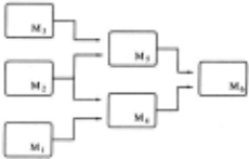
We performed some simple experiments to demonstrate the convergent behavior of our algorithm and to verify our ~ntu itions about the additive structure of MDP value functiOns. Figure 1 shows an abstracted factory with six machines, M1 ... M6 · In this problem, a machine can be in two states, working and not-working. If a machine and all of its prede cessors were working in the previous time step, then the ma chine will work in the current time step with probability 0.8. There is a stochastic startup lag, which reduces this probabil ity to 0.5 if the machine was not working in the previous time step. No machine can operate if its predecessors w~re n?t both working in the previous time step. Note that a fmlure m any of M1 ... M3 will have a cascade effect, ultimately caus ing M6 to fail. It will take several time steps for the sy~tem to recover. A reward of 1.0 is received whenever machme M6 is working.
We evaluated this 64-state system using our constrained value determination algorithm with a discount factor of 1 = 0.90 and a series of six different bases. The basis functions are binary so that, for example, h(M2 , Ml) has value 1 when both M2 and M1 are working, and value 0 otherwise. We per formed both unweighted projection, which is not guaranteed to converge, and our weighted projection algorithm. For this problem, we achieved convergence in all cases. The second and third columns of Table 1 show the reduction in error as new basis functions are added. The first three additions allow the value function to depend on the status of more individual machines. The last three allow it to depend in a correlated way on the status of pairs of machines. In each case, we approximated the stationary distribution using a product of dis tributions over the individual machine states. Notice that the weighted projection outperforms unweighted projection in all cases, even in the unweighted norm. Also, the p* weighted error for the weighted projection is monotonically decreas ing, while the other errors fluctuate. The final value function for the weighted projection with all ten basis functions corre sponds to an unweighted RMS error of less than 0.141. The true value function for this problem assigns values between 0.48 and 2.78, so that 0.141 is a very reasonable error bound. Hence, our final value function is a good 10 parameter ap proximation to the true, 64 parameter value function .
| Added basis | Unweighted Projection | Weighted Projection | ||
|---|---|---|---|---|
| functions | SSE'" | SSE. | SSE'" | SSEP. |
| 1, ~(Ma] | 1.449 | 1.663 | 0.260 | 0.303 |
| h(M5) , h(M4) | 0.319 | 0 .385 | 0.207 | 0 .174 |
| h(Ma) , h(M2), h(M,) | 0 .175 | 0.225 | 0.132 | 0.121 |
| h(M5 ,M4) | 0 .175 | 0.225 | 0.132 | 0.121 |
| h(Ms, M2) | 0.210 | 0.277 | 0 .120 | 0.115 |
| h(M2, Mt) | 0 .210 | 0.277 | 0 .120 | 0.115 |
To further verify our hypothesis about additive structure of value functions, we changed machine M6 so that it would work if either of M4 or M5 were functioning. In this case, we would expect the value function to be less sensitive to correlations between the status of M4 and M5 . The results, shown in the Table 2, support this hypothesis. We see that introducing the basis function h(M5 , M4 ) provides no sig nificant reduction in the error. (The overall increase in error compared to the original problem is probably due to higher overall values in this model- between 2.30 and 5.74.) We observe a similar pattern in the comparison of weighted and unweighted projection: weighted projection provides more reliable approximations.
Finally, we demonstrate how the value functions generated by our algorithm can be useful in decision making. Suppose that there are two types of workers, reliable and resilient. When a reliable worker is operating a working machine, it will continue to work properly with probability 0.9, but if the machine fails, the worker will restart the machine suc cessfully with probability 0.4. A resilient worker will keep a working machine functioning with a probability of only 0.8, but recovers from failures with probability 0.5. If the manager of our 6-machine factory has three of each type of worker, he may wish to compare different strategies for allocating workers to machines. One possibility would be a reliable first strategy that places the reliable workers on machines M1 ... M3 to avoid cascade failures. A resilient-first strategy would place the resilient workers on machines M1 ... M3 to recover quickly when failures occur. We consider the origi nal machine configuration, which requires both M4 and M5 to be working for machine M6 to work properly. For this problem the reliable-first strategy completely dominates the the resiliant-first strategy.
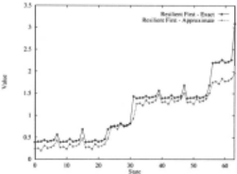
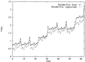
Figure 2 shows a graph of the true value function for the resilient-first strategy versus the approximation with all 10 basis functions. The states are numbered 0 ... 63. The status of the machines is used to identify the states, e.g., when ma chine M6 is working, the highest order bit of the state num ber has value 1; when machine M1 is working the lowest or der bit of the state number has value 1. Figure 3 shows both value functions for the reliable-first strategy. The qualitative closeness of the these approximations is apparent from in spection- the shape of the approximations are quite close to the shape of the exact value functions. Moreover the approx imate value functions maintain the dominance of the reliable first strategy over the resiliant-first strategy. Thus, we see that our approximation closely matches the qualitative structure of the exact value functions for these domains.
6 Policy evaluation
We now address the issue of using our value determination al gorithm to evaluate a policy in an MDP, where we extend the definition of our process to incorporate actions. Most impor tantly, the transition probability P and the reward R now also depend on a. In the context of factored MDPs, this extension is usually done by defining a separate transition graph and as sociated set of CPTs for each action a; the resulting transition probability Pa(X' I X) is thereby factored (perhaps in a dif ferent way) for every action a. The reward function can also vary over actions in a similar way.
Our goal now is to compute an approximate value function for a particular policy 1r. Intuitively, there seems to be no problem. A policy 1r in an MDP specifies a transition model Ptr(x' I x) and a reward function R1r(x). We might simply apply our algorithm to these. Unfortunately, the problem is somewhat more subtle. The most obvious difficulty is that the naive representation of a policy in an MDP with expo nentially many states is also exponentially large. Therefore, we might not even be able to construct a compact transition model and reward function for 1r . Clearly, we must restrict the set of policies that we consider to ones that can be efficiently manipulated by our algorithm.
To understand this issue, assume that we have constructed a value function v; t) , and are now trying to perform our DP and projection steps. We do not have a single transition model to use for the next step of backprojection, because the action depends on the state. However, we can use our algorithm to compute a factored approximation Q~t+ 1 ) to the Q function Qa(x) = Ra(x) + I I:x' Pa(x' I x)V; t): we simply back project v;t) through the transition model Pa, and then project into V. We now have to combine the different Q functions to get a complete value function . For each action a, Jet Sa be the subset of states in which a is taken, and let I sa be the in dicator function which takes value 1 at x when x E Sa and value 0 otherwise. Then,
We see that, depending upon the policy, V(t+l ) can be com posed of an arbitrary combination of pieces of the Q(t+l ) functions. In particular, if the indicator functions I sa depend on variables in many different clusters, the combination will no longer be in V, even if each of the Q<t+ 1 ) is in V. Thus, we need to project v <t+ 1 ) back into v.
As before, we need to compute ((!sa · v <t+ 1 l) · hj )p to perform the projection. This reduces to the problem of com puting ((I sa · Q(t+ 1 )) ·hj) p for each action and summing the results. Since Q(t+ 1 ) is in V, it can be represented as I:i Ui, where each Ui is restricted to some small cluster Ci. Again, we need only compute ((Isa · Ui) · hj )p· Let Y be the set of variables appearing in Ci u Ci. Then:
where Sa(Y] = {x E Sa : xis consistent withy} . Thus, in order to perform this weighted dot product operation, we must be able to compute the total probability, according to the approximate stationary distribution, of Sa(y]. In many cases, this computation is far from trivial, even if the set Sa has a simple and compact description (e.g., as a linear separator defined over the variables X 1 , ... , Xn).
However, for what is arguably the most often-used class of compactly represented policies, this computation can be done easily. 4 A region-based policy is one represented as a set { ( Zk , ak) }~=1 , where each ze is an assignment of values to some subset of the variables in X . (Different ze 's can refer to different sets of variables.) Each ze thereby specifies a region in the state space, such that action ae is taken in this region. The assumption is that the regions corresponding to the different ze are mutually exclusive and exhaustive. Note that a decision tree representation of the policy [Boutilier and Dearden, 1996], falls into this category, as do the policies for the aggregated state spaces [Dean et al., 1997]. Given the factored representation of p, p(ze, y) can be computed simply and efficiently, in the obvious way.
4 For other classes of policies, Monte Carlo sampling may suc ceed in providing good estimates for p(Sa[y]) . We defer discussion to a longer paper.
It remains only to extend the algorithm of BK to the task of computing the approximate stationary distribution, p, for a region-based policy, 1r. Recall that their algorithm was based on repeatedly computing a factored belief state p,(t+l) from a factored belief state p,<t l, where
Here, we have a potentially different transition model Pat for each ae. Therefore, we must do a separate computation for each of them:
Fortunately, the algorithm of BK can easily be adapted to this task. We simply instantiate ze as evidence into the Bayesian network that they use for doing the one step propa gation, and then compute the internal summation. The prob abilities p,(t) (ze) can be computed easily, as described above. This algorithm provides a factored representation of the sta tionary distribution, which can be used in Equation 4. Thus, we can efficiently compute an approximate value function for any region-based policy.
7 Discussion and conclusions
We have shown that we can efficiently compute factored ap proximations to value functions. We have also demonstrated, both theoretically and empirically, that the result of our ap proximate value determination algorithm can often be quite close to the true value function. Finally, we showed how to use our algorithm for evaluating policies in a restricted but interesting class.
It is useful to compare our algorithm to other algorithms for factored MDPs [Boutilier et al. , 1999]. Some algorithms for factored MDPs try to construct compact value functions by exploiting structured, usually tree-based, CPTs. When the value function representation becomes too large, the standard approach is to perform a type of state aggregation [Boutilier and Dearden, 1996; Dean et al., 1997]. Thus, their approxi mate value function is one that is piecewise constant over the state space. In other words, there are substantial blocks of states all of which take the same value. A main advantage of our approach is that it uses a richer class of value function approximations. It seems clear that, at least in some domains, a linear approximation is much more accurate. While the al gorithm presented in this paper does not exploit structured CPTs, this feature can be added easily to make both the dy namic programming steps and projection steps more efficient.
Other approaches [Meuleau et al., 1998; Boutilier et al., 1998; Singh and Cohn, 1998] decompose the process into subprocesses, and compute a separate value function for each one. They then attempt to combine the different value func tions into a global one using some heuristic approximation. Generally speaking, the decoupling of the process is a much harsher approximation than the factorization of the value function. The latter still allows influence to flow between the different subprocesses, and thereby is likely to get more ac curate results.
Of course, it is important to remember that these other ap proaches solve the planning problem whereas, at least for now, our algorithm is restricted to the value determination problem. The obvious question is how our value determina tion algorithm can be used for planning. The most obvious approach is to use our algorithm as a subroutine in an algo rithm such as policy iteration, where we compute the value function for some policy, and use it as guidance for locally improving the policy. Unfortunately, there are barriers to this application of our algorithm. The difficulty lies in the nature of our approximation. We measure our distance from the true value function in a norm that is weighted by the probability that the different states will be visited in the stationary dis tribution. Hence, states that are visited infrequently can have very poor value estimates. Changes to the policy based upon these estimates will not be guaranteed to improve the overall policy as in exact policy iteration, and could actually make the policy much worse. The issue of using our value func tions as guidance in policy search is an important direction for future work.
There are, however, several other important uses for a value determination algorithm. Plan evaluation is an important problem in and of itself; our algorithm allows us to take poli cies generated by a user or some other tool, and produce a fairly good value function for them. Furthermore, it is known that simple policies can be improved significantly by the ad dition of a smalllookahead search that uses the value function of the policy as a heuristic value at the leaves of the search. Indeed, the recent work of Sutton [ 1999] shows that even very simple policies can be quite powerful if a meta-level reasoner is allowed to choose which one to apply in different contexts. Our algorithm can readily be used to compute the value func tions necessary for making such a choice.
Factored MDPs provide us with a compact and natural rep resentation for the type of complex problems that arise in real world settings. Unfortunately, the structure is not reflected in the value function for these processes. However, we believe that the value functions that arise are often approximately factored, i.e., approximated well by the generalized additive functions that we have discussed. The fact that such functions are often used by human decision makers supports this intu ition. We therefore believe that algorithms that exploit this structure can be very successful. This paper takes a first step towards this goal.
Acknowledgement
We are grateful to Craig Boutilier, Andrew Ng, Satinder Singh, and Benjamin Van Roy for helpful discussions. This work supported by ARO grant DAAH04-96-l-0341 under the MURI program "Integrated Approach to Intelligent Sys tems", by ONR contract N66001-97-C-8554 under DARPA's HPKB program, and by the generosity of the the Powell Foundation and the Sloan Foundation.
@inproceedings{ijcai1999p189,
  title     = {Computing Factored Value Functions for Policies in Structured MDPs},
  author    = {Koller, Daphne and Parr, Ronald},
  booktitle = {Proceedings of the Sixteenth International Joint Conference on
               Artificial Intelligence, {IJCAI-99}},
  publisher = {International Joint Conferences on Artificial Intelligence},
  editor    = {Thomas Dean},
  pages     = {1332--1338},
  year      = {1999},
  note      = {Uncertainty and Probabilistic Reasoning},
  url       = {https://ijcai.org/proceedings/1999/189},
}
TY - CPAPER TI - Computing Factored Value Functions for Policies in Structured MDPs AU - Koller, Daphne AU - Parr, Ronald T2 - Proceedings of the Sixteenth International Joint Conference on Artificial Intelligence, IJCAI-99 PB - International Joint Conferences on Artificial Intelligence PY - 1999 SP - 1332 EP - 1338 UR - https://ijcai.org/proceedings/1999/189 ER -Copied
Machine-readable versions of this paper, for tools and AI agents:





