Decomposition Techniques for Planning in Stochastic Domains

1 Introduction

We are concerned with solving planning problems posed as Markov decision processes. Specifically, given a dy­ namical model described as a stochastic process (e.g., Markov chain) with a large, discrete state space and a performance criterion (e.g., minimize the expected time or cost to reach a goal), construct a policy (plan) map­ ping states to actions that realizes the specified perfor­ mance criterion or approximates it to within some spec­ ified tolerance.

*This work was supported by the Air Force and the Ad­ vanced Research Projects Agency of the Department of De­ fense under Contract No. F30602-91-C-0041, and by the Na­ tional Science Foundation in conjunction with the Advanced Research Projects Agency under Contract No. IRI-8905436.

1.1 Factoring Large State Spaces

Large state spaces present a number of challenges. To begin with, the problem has to be efficiently encoded. A factored state-space representation uses state variables to represent different aspects of the overall state of the system. 1 Compact encodings for stochastic processes can be achieved for many applications using factored state-space representations, where the size of the model is usually logarithmic in the size of the state space [Dean and Kanazawa, 1989]. Similarly, policies for large fac­ tored state spaces can often be efficiently encoded using decision trees that branch on state variables [Boutilier et al., 1995]. Assuming that both the problem (a stochastic process) and the solution (a policy) can be encoded in a compact form, we would like to generate solutions in time bounded by some small factor of the problem and solution size.

1 Propositions representing fluents in STRIPS operators [Fikes and Nilsson, 1971] correspond to state variables in a factored state-space representation.

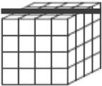
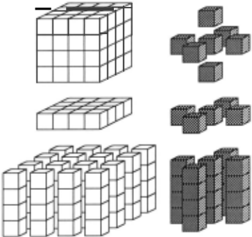
A factored state-space representation with n boolean state variables represents an n-dimensional state space with 0(2n) states. We assume that all of the state vari­ ables are relevant in at least some portion of the state space and so the dimensionality of the problem cannot be reduced without suffering some loss in performance. However, it is very likely that not all state variables are relevant in all portions of the state space (e.g., when you are planning to take a walk in southern Florida you can neglect the possibility of snow). Figure 1 illustrates three views of a multi-dimensional state space. The bot­ tom view in which the state space is partitioned into aggregate states is the view we are most interested in.

1.2 Dimensionality Reduction

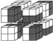
In this paper, we assume that a domain expert has par­ titioned the state space into m regions such that in each region only a small subset (of size no more than r, r « n) of the set of all state variables is relevant for decision making. In other words, for each region, we are con­ cerned with an abstract subspace of size no more than 2r. The size of the union of these abstract subspaces is no more than m2r. The problem of automatically constructing such a partition is not addressed in this paper, but see [Lin and Dean, 1994] for some relevant techniques. Figure 2 illustrates how a three-dimensional state space might be represented as the union of two­ dimensional abstract subspaces.

There exist methods for computing policies that are polynomial in the size of the state and action spaces [Papadimitriou and Tsitsiklis, 1987] [Puterman, 1994], but these methods are impractical for large state spaces (e.g., > 10 6 states, given 20 state variables). Instead of considering the large state space as a whole, we are interested in decomposition methods that deal with the smaller subspaces of individual regions.

1.3 Combining Local Solutions

Our framework is a special case of divide and conquer: given a Markov decision process and a partition of the state space into regions, (i) reformulate the problem in terms of smaller Markov decision processes over the sub­ spaces of the individual regions, (ii) solve each of these subproblems, and then (iii) combine the solutions to ob­ tain a solution to the original problem.

In the best case, all of the subproblems are indepen­ dent and combination is trivial (e.g., a manufacturing task that involves assembling and testing several com­ ponents each of which is assembled independently). In such cases, it does not matter how you enter a region of the partition or how you leave; the only thing that matters is the cost accrued while in that portion of the state space. In the more likely case, the subproblems are weakly coupled to one another so that, for example, what you do in one region only affects what you do in a few neighboring regions. Examples ofweakly-coupled systems include staged manufacturing and military plan­ ning problems and robot navigation tasks.

We associate a set of topologically motivated param­ eters with each region R. These parameters summarize the interactions between R and the other regions in the partition. A specific estimate of the parameter values as­ sociated with region R allows us to construct a Markov decision process over the subspace associated with R. By solving such a Markov decision process, we deter­ mine a local policy on the region R, which is a solution to the subproblem associated with R. In this paper, we describe two basic methods for combining solutions to subproblems in order to generate a solution to the global problem.

The first combination method is illustrated in an algo­ rithm called hierarchical policy construction, which con­ siders particular sets of parameter values that have an intuitive topological interpretation. These sets of pa­ rameter values give us a set of candidate local policies associated with each region. We then construct an ab­ stract Markov decision process by considering individual regions as abstract states and their candidate local poli­ cies as abstract actions. The solution to this abstract Markov decision process assigns a particular candidate policy to each region, thus yielding a policy on the en­ tire state space. Hierarchical policy construction pro­ duces an optimal policy only in special cases; however , it does so relatively efficiently and has an intuitive in­ terpretation that makes it particularly suitable for robot navigation domains.

The second method of combining solutions involves it­ erative approximation of the optimal parameter values, i.e., those values associated with optimal solutions to the global problem. On each iteration of the iterative approximation method, we consider for each region R, a specific estimate of the parameter values for region R, and solve the resulting Markov decision process to ob­ tain a local policy. By examining the resulting local poli­ cies, we obtain information to generate a new estimate of the parameter values that is guaranteed to improve the global solution. This information about local poli­ cies also tells us when the current solution is optimal or within some specified tolerance, and therefore when it is appropriate to terminate the iterative procedure.

1.4 Overview of the Paper

In Section 2, we provide a brief introduction to Markov decision processes. Section 3 describes the parameters modeling the inter-regional interactions, and the con­ struction of a Markov decision process on a region R given a specific estimate of the parameter values for R. Section 4 presents the hierarchical policy construction algorithm. We describe the construction of abstract de­ cision processes from a base-level process, and the use of such abstract decision processes to construct policies for the base-level process. Section 5 illustrates the method of the iterative approximation and briefly addresses is­ sues concerning convergence, optimality, and complex­ ity. Details are available in a longer version of the paper [Dean and Lin, 1995].

2 Markov Decision Processes

Let M = (Ox, DA, p, c) be a Markov decision process with finite state space Dx, actions nA, state transition matrixp, and cost matrix c. Let Dx = {1, 2, ... , N}. Xt (At) is a variable indicating the state (action) at timet. For all i,j E Dx and a E DA, we have

where Pr(.l.) is a conditional probability distribution and C(.l.) is a real-valued cost function. A policy 1r is a function mapping states to actions 7r : Dx -+ nA.

To completely define a Markov decision process we also need a performance criterion. Two criteria that we consider are expected discounted cumulative cost and ex­ pected cost to reach a specified goal. In the former, the task is to find a policy minimizing the expected cumula­ tive cost function,

for all i E Dx where 0 < 1 < 1 is the discount rate, E 1 represents the discounted cumulative cost, and Err(·l·) denotes an expectation with respect to the policy rr. For the criterion of expected cost to reach a specified goal, a subset of Dx is designated as a target and perfor­ mance is measured as the expected cost until arriving in some target state. Informally, we can model each tar­ get state as a sink (all transitions out have probability zero, Pi#i (a) = 0) and proceed as in the case of expected discounted cumulative cost but with 1 = 1.

We mention two standard methods for solving Markov decision processes. Bellman's value iteration method [Bellman, 1961] iterates by .computing the optimal ex­ pected cumulative cost function accounting for n steps of lookahead using the optimal expected cumulative cost function accounting for n-1 steps of lookahead. Value it­ eration is guaranteed to converge in the limit to the opti­ mal expected cumulative cost function accounting for an infinite lookahead. Howard's policy iteration [Howard, 1960] iterates by first computing the expected cumula­ tive cost function for the current policy and then im­ proving the policy by using this cost function. Policy iteration is guaranteed to converge to the optimal pol­ icy in time polynomial inN. Puterman [1994] provides an up-to-date overview of algorithms for solving Markov decision processes.

In iterative methods, it is often useful to be able to compute a bound on the difference between the value of the current solution and the optimum. Let rr* denote an optimal policy for M. Suppose ~; is the probability of starting out in state i and 1r is the current policy then l:iEOx ~;Err (.E,Ii) is the value of the current solution and L::iEO ~;Err· (E1 Ii) is the optimum. The algorithm described in Section 5 relies on computing such a bound.

3 Decomposing Markov Processes

In this section, we describe a general method of de­ composing a Markov decision process defined on a large state space into smaller Markov decision processes de­ fined on local regions. Based on this regional decom­ position framework, we develop two approaches in the following two sections that combine the solutions to the smaller Markov decision processes into a solution to the original Markov decision process.

Let P be any partition ofDx, P = {Rl> ... , Rm} such that Dx = U;: 1 R; and R; n Rj = 0 for all i f= j. We refer to a region R E P as an aggregate state. We refer to a state in Dx as a base-level state.

The periphery of an aggregate state R (denoted Periphery ( R)) is the set of all base-level states not in R but reachable in a single transition from a base-level state in R, {jlj f/. R 1\ 3i E R,a E DA,Pij(a) > 0}. We say that aggregate state R in P is adjacent to aggregate state S in P (denoted R--.....S) just in case Periphery(R) nSf= 0.

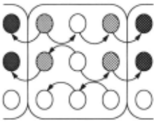
The boundary of an aggregate state R (denoted Boundary(R)) is the set of all base-level states in R from which you can reach a base-level state not in R in a sin­ gle transition, {iii E R 1\ 3j f/. R, a E DA, Pij(a) > 0}. In Figure 3, the boundary states are shaded light gray and the periphery states are shaded darker gray.

Next, we introduce a set of parameters that we will use to model interactions among regions. Let U = UREP Periphery(R), and A; for each i E U denote a real-valued parameter. Let .X E :RIUJ denote a vector of <.'1:11 such A; parameters, and .XIR denote a subvector of A composed of A; where i is in Periphery (R). U is the medium for inter-regional interactions; a region R can only communicate with the other regions through the states in U. Parameter A; serves as a measure of the expected cumulative cost of starting from a periphery state, and .XIR provides an abstract summary of how the other regions affect R.

Given a particular .X, the original Markov decision process can be decomposed into smaller Markov deci­ sion processes, each of which determines a local pol­ icy on a local region. For a region R and the sub­ vector 5.iR of >., we define a Markov decision process MxiR = (RUPeriphery(R), nA, q, k) and the correspond­ ing local policy rrx 1 R as follows.

1. RUPeriphery(R) is the (local) state space for Mx 1 R.

1. Qij is the (local) state transition matrix for M;; 1 R, where
2. Qij = Pij for i E R
3. q;; = 1 for i E Periphery(R)
4. k;j is the (local) cost matrix for M;; 1 R, where
5. k;j = c;j for i, j E R
6. k;j = Aj + c;j for i E Rand j E Periphery(R)
7. k;; = 0 for i E Periphery(R)
8. 1l'>;JR corresponds to the local policy that is optimal for M;; 1 R with performance criterion expected cost to goal and target set Periphery(R).

M;; 1 R is the subproblem we associate with region R given >-iR as an abstract summary of R's interaction with the other regions. 1l'>;JR is the solution to the subproblem M;; 1 R. A particular >. determines a set of local policies (abstract actions) which in turn determines a policy on the entire state space. Let 7r* denote an optimal policy forM. If>..; = E1r· (:E-y li), then the resulting local policies as defined above define an optimal policy on the entire state space. The algorithms considered in the following two sections offer various methods for either guessing or successively approximating E1r· (E-y li) for all i E U.

4 Hierarchical Policy Construction

In this section, we first describe a general method for constructing an abstract decision process from a base-level process given a fixed partition of the state space. We then present a hierarchical policy construc­ tion method for using an abstract decision process to construct policies for the base-level process.

4.1 Abstract Decision Processes

Let P = {R11 ... ,Rm} be any partition of f2x. Each region R E P is considered as an abstract state. A par­ ticular local policy 1l'>;JR on region R is considered as an abstract action on R, which reflects our bias toward different periphery states described by >-iR· Abstract ac­ tions for stochastic domains are the rough equivalent of macro operators for deterministic domains. The abstract action 1l'>;JR indicates how to act optimally in region R if the interactions with the other regions are captured in >.. For example, a large value for >..j naturally discourages us from entering the periphery state j since it induces a large cost in k;j. The family of all abstract actions is denoted :F = {7r>;JR IRE P, >. E RJUI}.

The probability of ending up in S starting in R and following an abstraction 1l'5;J R is defined by

where Pij = Pij(11';; 1 R(i)). Note that we assume here that there is an equal probability of starting in any state in the boundary of R.

The cost of ending up in S starting in R and following 1l'>;JR is defined by

where c;j = c;j(11'>;JR(i)).

The resulting abstract decision process is then defined by M;; = (P,:F,p',c'). It is important to note that M>-. need not be Markov; in some cases, we may simply ac­ cept this as one of the inevitable consequences of ab­ straction and proceed as if the process is Markov; in other cases, we may attempt to ameliorate this condi­ tion (at some increase in computational cost) by using one of several standard techniques.

4.2 Hierarchical Policy Construction

In the following algorithm, called hierarchical policy con­ struction, we restrict our attention to a finite subset of :F. For each R and each S adjacent to R, we construct a local policy 1l'R--+S by setting >..; = 0 fori E S n Periphery(R) and setting >..; = K for i E Periphery(R) - S, where K is some fixed constant. If the performance criterion for the base-level process is expected cost to goal, then for each R containing one or more target states, we add an additional action in which all the peripheral states get >..; = K and all of the target states are made into sinks with k;; = 0. The abstract decision process is (P,:F,....,p',c') where :F,.._. = {7rR--+siR,S E PI\R"-'S} and the performance criterion is expected discounted cu­ mulative reward for a discount rate I·

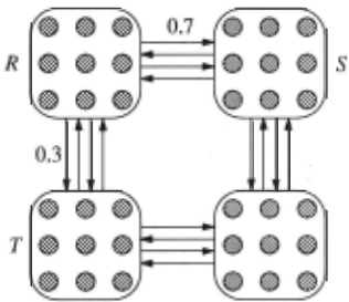
The local policies have the interpretation that 1l'R--+S is the policy to take starting in R if you want to get to S. The larger K is, the more incentive there is to get to S and avoid the rest of the periphery of R. Figure 4 illustrates an example in which P~s(1l'>;JR) = 0.7 and P~T(1l'>;JR) = 0.3. The abstract policy has the interpre­ tation of providing a global perspective and indicating for each region the best local policy to use. Generally, it is best to set 1 very close to one or use an alternative performance criterion such as average expected cost per step [Derman, 1970].

The following is an algorithm to construct a global policy using the abstract decision process (P, :F-..., p', c').

1. Set K and compute 7rR-+S for R"'-'>S E P.
2. Calculate the abstract transition probabilities p' and abstract costs c'.
3. Set 1 and solve the abstract decision process to ob­ tain an abstract policy n : p -+ :F "'-+.
4. To determine the action to take in base-level state i, determine R E P such that i E R and take action TI(R)(i).

The above algorithm for constructing and solving ab­ stract processes can be applied recursively and hence applies to hierarchical partitions.

Hierarchical policy construction produces an optimal policy only in special cases; however, it does so rela­ tively efficiently and has an intuitive interpretation that makes it particularly suitable for robot navigation do­ mains. For a simple partition of the state space with no aggregation within regions, standard algorithms [Puter­ man, 1994] on the base-level state space would be domi­ nated by a factor quadratic in the size of the state space (lOx/) , while hierarchical policy construction would be dominated by the number of regions in the partition (IP/) times the maximum number of neighbors for any region (maxREP I{SIS E P 1\ R"'-'>S}/) times the square of the size of the largest region (maxREP IRI).

5 Iterative Improvement Approach

Given a particular 5., the base-level process is decom­ posed into local processes, {Mx 1 R}. By solving these lo­ cal processes, we derive the corresponding local policies (abstract actions) {rrx 1 R}. The solution policy, rr, to the ba.Se-level process is then derived by combining these lo­ cal policies together. The quality of rr critically depends on the choice of 5.. Instead of relying on a particular 5., we can successively modify 5. and proceed through multiple iterations of decom.position and localized com­ putation to determine a policy for the base-level process. There are three issues in realizing this iterative improve­ ment framework:

• how to modify 5. iteratively so that the solution quality can be improved on each iteration and is guaranteed to converge to an optimal solution in a finite number of iterations,
• how to determine it is time to terminate the compu­ tation when the solution is optimal or within some specified tolerance, and
• how to combine the previously generated local poli­ cies into a policy of the base-level process when we terminate the computation.

In this section, we focus on a particular iterative method that resolves these three issues. This itera­ tive method is based on a reduction to the methods of Kushner and Chen [1974] that demonstrate how to solve Markov decision processes as linear programs using Dantzig-Wolfe decomposition [Dantzig and Wolfe, 1960].

The details of the material presented in this section depend on some understanding of linear programming [Chvatal, 1980] and methods for decomposing and solv­ ing large systems [Lasdon, 1970]. Rather than assume this understanding, we refer the reader to the longer ver­ sion of the paper [Dean and Lin, 1995] for the details and just sketch the method in the following.

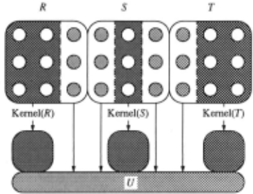
1. Given an arbitrary partition P = { R,, ... , Rm} of size m, we first transform P into a new partition Q = {To, T,, ... , Tm} of size m + 1 as follows. For each region R define Kernel(R) to be R - U (re­ call that U = UReP Periphery(R)). Q is defined by To = U and T; = Kernel(R;) for 1 ~ i ~ m. The resulting structure induces a star topology that is critical in arplying the techniques in [Kushner and Chen, 197 4 . To = U is called the coupling region; removing the states in To separates the state space into isolated regions, each of which corresponds to a T;, i > 0. Figure 5 illustrates the relationship between the partitions P and Q.
2. In the ith iteration, we consider the particular 5. de­ termined at the end oflast iteration. We decompose the original base-level process into local processes { Mx1R IR E Q}, and derive the corresponding local policies { rrx1R IR E Q}. Let TI; denote the global policy formed by gluing together these local poli­ Cies.
3. We need to maintain a policy repository of at most lUI+ 1 previously generated global policies at a time. As soon as policy TI; is generated, it replaces some policy Tij, j < i, in the repository. The information associated with the current policy repository tells us an upper bound on the gap between the value of the current solution and the optimum. This bound allows us to determine whether we have reached the optimum or are within a specified range of the opti­ mum, and whether we should continue for another iteration or terminate and report a final solution.
4. If we decide to terminate the computation, we gen­ erate a policy as a final solution by properly com­ bining the policies in the current policy repository using its associated information; otherwise, we de­ termine a new 5. according to the information asso-

ciated with the current policy repository.

Proposition 1 The iterative method described above im­ pmves the solution quality on each iteration, and con­ verges to an optimal solution in a finite number of steps.

For a proof of this proposition and a more detailed description of the algorithm see the longer version of this paper [Dean and Lin, 1995]. Our approach to anal­ ysis involves (i) reformulating this iterative method in terms of solving large linear programs, and (ii) applyin& a reduction to the methods of Kushner and Chen [1974j that solve these large linear programs for Markov de­ cision processes using Dantzig-Wolfe decomposition. In the following, we briefly discuss the convergence rate and the time and space complexity of this iterative method.

• Empirical experience suggests that the Dantzig­ Wolfe method of decomposition upon which our analysis of the iterative method is based converges to within 1- 5% of the optimum fairly quickly, al­ though the tail convergence rate can be very slow (see page 325 in [M.S. Bazaraa, 1990]). In other words, it is likely that after only a small number of iterations in the iterative method we are able to produce a solution of good quality, but it may not be worthwhile to continue after reaching 1-5% of the optimum.
• The computational task in an iteration is decom­ posed into two subtasks: (i) deriving and solving local processes over local regions as subproblems, and (ii) maintaining a policy repository of up to lUI + 1 previously generated policies, where U is the union of Periphery(R) for the regions R in the original partition P.

The computational cost in an iteration is critically affected by the structure of the partition Q: (i) the maximum number of base-level states in a region in the partition Q, and (ii) lUI, the total number of base-level states in the coupling region for the partition Q.

• Compared with solving the original base-level pro­ cess as a whole, the first subtask can be achieved more efficiently by applying the standard techniques for Markov decision processes over individual re­ gions. This is a natural advantage of decomposi­ tion techniques, which divide large problems into subproblems of tractable size.

The second subtask is achieved by maintaining a (lUI+ 1) x (lUI+ 1) matrix, whose computational efficiency critically depends on the topology of the given partition P. The second subtask can be per­ formed efficiently if the size of U is relatively small. This is the additional cost to pay for decomposition techniques since we need to combine the solutions to subproblems.

• In other words, this iterative method is promising if the given partition P evenly divides the whole state space into many regions, and the number of states in the peripheries of the regions in P is small.

In the longer version of this paper, we also describe other iterative methods that do not necessarily converge to an optimal solution but allow intuitive interpretation and more computational efficiency. We are currently testing these algorithms on a set of benchmark problems. Since the discussion is somewhat lengthy and requires some understanding of both Howard's policy iteration [Howard, 1960] and Bellman's value iteration [Bellman, 1961] for solving Markov decision processes, we refer the interested reader to the longer version of the paper [Dean and Lin, 1995].

6 Related Work

The related work on abstraction and decomposition is extensive. In the area planning and search assuming de­ terministic action models, there is the work on macro operators [Korf, 1985] and hierarchies of state-space op­ erators [Sacerdoti, 197 4] [Knoblock, 1991]. Closely re­ lated is the work on decomposing discrete event systems modeled as (deterministic) finite state machines [Zhong and Wonham, 1990] [Caines and Wang, 1990].

In the area of reinforcement learning, there is work on deterministic action models and continuous state spaces [Moore and Atkeson, 1995] and stochastic models and discrete state spaces [Kaelbling, 1993]. The hierarchica l policy construction method described in Section 4 pro­ vides an alternative formulation of Kaelbling's hierar­ chical learning algorithm [Kaelbling, 1993] and suggests how Moore and Atkeson's parti-game algorithm might be extended to handle discrete state spaces.

The analysis hinted at in this paper and found in the longer version of the paper borrows heavily from the work in operations research and combinatorial optimiza­ tion for representing Markov decision processes as lin­ ear programs [D'Epenoux, 1963] [Derman, 1970] [Kush­ ner and Kleinman, 1971] and decomposing large sys­ tems generally [Dantzig and Wolfe, 1960] [Lasdon, 1970] and Markov decision processes specifically [Kushner and Chen, 1974]. The approach described in [Dean et al., 1993] [Dean et al., 1995] represents a special case of the framework presented here, in which the partition con­ sists of singleton sets for all of the states in the envelope and a set for all the states in the complement of the envelope.

7 Conclusion

The benefit of decomposition techniques is that we are able to deal with subproblems of smaller size; the trade­ off is that extra effort is required to combine the solu­ tions to these subproblems into a solution to the original problem. The leverage of decomposition techniques is or­ thogonal to that of standard techniques used to solve the original problem. In the case of problem instances of very large size, decomposition techniques are often valuable even if standard polynomial-time algorithms are avail­ able.

We provide decomposition techniques for Markov de­ cision processes, given an arbitrary partition of the state space into regions. Subproblems correspond to local M~1.rkov decision processes over regions associated with a A parameter that provides an abstract summary of the interactions among regions. We present two methods for combining the solutions to subproblems: a hierarchical construction approach and an iterative improvement ap­ proach. The hierarchical construction method provides a quick solution with an intuitive interpretation. The it­ erative method is guaranteed to converge to an optimal solution in a finite number of iterations. For practical purposes, a small number of iterations should be suffi­ cient for a solution of near optimal quality.

Acknowledgements

We thank Craig Boutilier, Moises Goldszmidt , Steve Hanks, David Smith, and Mike Williamson for their com­ ments on the content and presentation of the ideas de­ scribed in this paper.