Variable Resolution Discretization for High-Accuracy Solutions of Optimal Control Problems

1 Introduction

This paper is about non-uniform discretization of state spaces when finding controllers for continuous optimal control problems. Uniform discretizations suffer from impractical computational requirements when the size of the discretization step is small. In this paper we try to keep the convergence properties of the discretization methods while introducing a variable resolution approx­ imation . Here, we only consider the "general towards specific" approach : an initial coarse grid is successively refined at some areas of the state space by using a split­ ting process, until some desired measure of accuracy is reached.

We consider discounted deterministic control prob­ lems, which include the well-known reinforcement learn­ ing (RL) benchmarks of "car on the hill" [Moore, 1991], Cart-Pole [Barto et al., 1983] and Acrobot [Sutton, 1996a]. Let x(t) E X C IR be the state of the system whose evolution is described by the controlled differen­ tial equation :

The objective of the control problem is to find, for any initial state x, the control u*(t) that optimizes the gain:

where r(x , u) is the current reinforcement, R(x) the boundary reinforcement (obtained at the boundary of the state-space) , 1 the discount factor ( 0 :S 1 < 1) , and T the exit time from X. The value function (VF), max­ imal value of the gain, is :

It is known (see [Fleming and Soner, 1993]) that V sat­ isfies a first-order non-linear differential equation, called the Hamilton-Jacobi-Bellman (HJB) equation :

with DV being the gradient of V .

Section 2 introduces the discretization process ; sec­ tion 3 describes several local splitting criteria, based on the value function and on the policy ; and section 4 proposes a heuristic for a global splitting criterion.

2 The discretizat ion p rocess

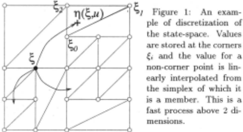
The state-space is discretized into a variable resolution grid using a structure of a kd-tree. The root of the tree covers the whole state space, supposed to be a (hyper) rectangle. Each node (except for the leaf nodes) splits in some direction the rectangle it covers at its middle into two nodes of half area. For each leaf, we use a Kuhn triangulation to linearly interpolate inside the rectan­ gle (see the triangulation of figure 1). See [Munos and Moore, 1999] for more details. This defines a class of functions known as barycentric interpolators [Munos and Moore, 1998] which are piecewise linear , continuous in­ side each rectangle, but may be discontinuous at the boundary between two rectangles .

The discretization process is based on the finite­ element methods of [Kushner and Dupuis, 1992] (ex­ tended to RL in [Munos, 1999]) which approximate, for any given discretization of the state space, the continu­ ous deterministic control process by a Markov Decision Process (MDP). Note that the stochastic aspect of the MDP does not come from the continuous problem itself (which is deterministic here), but from the discretization process used.

2.1 Building the discretized MDP

For a given discretization, we build the corresponding MDP in the following way. The state-space is the set 3 of corners of the tree. For every corner ~ and control u, we approximate a part of the corresponding trajec­ tory x(t) by integrating the state dynamics (1) from initial state ~ for a constant control u , during some timer(~ , u) until it enters inside a new simplex at some point TJ(~, u) (see Figure 1) . At the same time, we also compute the integral of the current reinforcement : R(~ , u) = ft~~ , u) --l.r(x(t), u).dt.

Then we compute the vertices (~0 , ... , ~d) of the simplex containing TJ(~ , u) and the corresponding barycentric co­ ordinates A{o(TJ(~ , u)) , ... , A{d(TJ(~ , u)) (which , by defini­ tion , satisfy: I:{; A{;(TJ) = 1 and I:{; A{;(TJ)('T]-~; ) = 0). The interpolated value at -'TJ(~, u) is thus just a linear combination of the values at the vertices ~0 , ... , ~d of the simplex it belongs to, with positive coefficients that sum to one. Doing this interpolation is mathematically equiv­ alent to probabilistically jumping to a vertex. Thus, we define the probabilities of transition p(~; I~ , u) of the MDP from state ~ and control u to states ~i as these barycentric coordinates : p( ~;I~, u) = A{; ( TJ( ~, u)), and the dynamic programming (DP) equation corresponding to this MDP is :

2.2 The "Car on the Hill" example

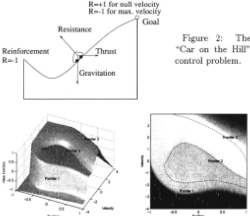
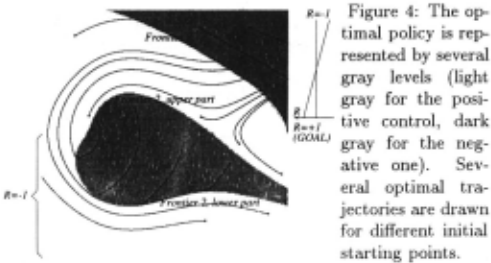
This problem, which will be made available on the web, is of 2 dimensions : position and velocity of the car. Here, the current reinforcement r( x, u) is zero everywhere. The terminal reinforcement R(x) is -1 if the car exits from the left side of the state-space, and varies linearly be­ t ween + 1 and -1 depending on the velocity of the car when it exits from the right side of the state-space. The best reinforcement +1 occurs when the car reaches the right boundary with a null velocity (see Figures 2 and 4). The control u has only 2 possible values : maximal positive or negative thrust. Because of the discount fac­ tor, we are encouraged to get to the goal as quickly as possible.

,.....,

Figure 3: The value function of the Car-on-Hill. Frontier 1 shows the discontinuity of the VF. Frontiers 2 and 3 (the dash lines) stand where there is a change in the optimal control.

Figure 3 shows the value function of this problem. The discontinuity along Frontier 1 happens because a point beginning just above the frontier can eventually get a positive reward whereas any point below is doomed to exit on the left. Note that there is no change in the optimal control around this frontier . There is a discon­ tinuity in the gradient of the VF along the upper part of Frontier 2 and along Frontier 3 because of a change in the optimal control.

2.3 The variable resolution approach

The basic idea is to start with an initial coarse discretiza­ tion, build the corresponding MDP, solve it in order to have a (coarse) approximation of the value function ; then refine locally the discretization by splitting rect­ angles according to some "splitting criterion", build the new MDP, and so on (see the splitting process in Fig­ ure 5) , until we estimate that the approximation of the value function or the optimal control is precise enough. The central purpose of this paper is the study of several possible splitting criteria.

3 Local splitting criteria

3.1 First criterion : average corner-value difference

For every hyper-rectangle in the tree we can ask the ques­ tion "do the values on the left-side of the rectangle tend to have a significantly different value on average than those on the right-side?". The notion of left and right depend on which axis we are considering splitting on, and in fact we iterate over all axes, finding the one with the most significant difference, which we will call the "corner-value difference".

Having computed this for all cells in the current tree, we must choose which cells to actually split. We select some fraction (e.g. 50%) of the cells with the highest criterion values and break them in half along their most significant splitting directions . Figure 6 represents the discretization obtained using this criterion.

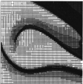
Figure 6: The dis­ cretization of the state­ space for the Car-orr­ Hill problem obtained after 15 splitting itera­ tions, starting with a 9 by 9 initial grid and us­ ing the corner- value dif­ ference criterion with a splitting rate of 50% of the rectangles at each iteration.

3.2 Second criterion : value non-linearity

For every rectangle, we compute the variance of the ab­ solute increase of the values at the corners of the edges for all directions i = O .. d. This criterion is similar to the previous criterion except that it measures the extent to which the value throughout the cell is non-linear in­ stead of non-constant. Figure 7 shows the corresponding discretization.

The value non-linearity criterion splits more parsimo­ niously than corner-value difference because it intends to refine whenever the approximated function is non-linear instead of non-constant (see the difference of splitting in the area above the frontier 3, where the value function is almost linear) .

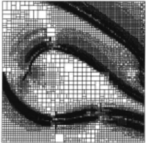
We observe that in both cases, the refinement process does not split around the bottom part of frontier 2, be­ cause the VF is almost constant in this area although there is a change in the optimal control.

We observe that in both of these splitting processes based on the approximation of the VF, there is a huge amount of memory spent for . the approximation of the discontinuity despite the optimal control being constant in this area. This is undesirable and so in the next sec­ tion we will pay attention to the policy when splitting.

3.3 The policy disagreement criterion

Figure 4 shows the optimal policy and several optimal trajectories for different starting points. We would like to define a process that could refine around the areas of change in the optimal control, that is around frontiers 2 and 3, but not around frontier 1.

When we solve the MDP and compute the value func­ tion of the DP equation, we can compare the policy given by the arg maXu of equation ( 4) with the optimal control law derived from the local gradient of V (given by the arg max,. in equation 3) . We define the states of policy disagreement being those where these two measures of the optimal control diverge.

Figure 8 shows the discretization obtained by splitting the rectangles containing states of policy disagreement .

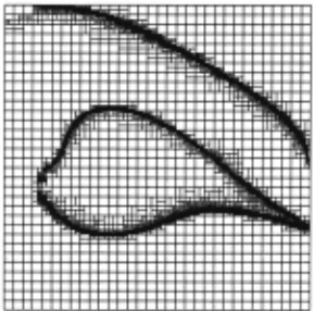
Figure 8: The discreti­ zation of the state-space for the Car-on-Hill usment criterion (Here we used an initial grid of 33 x 33 and a splitting rate of 20% to obtain this discretization) .

This criterion is interesting since it splits at the places where there is a change in the optimal control, thus re­ fining the resolution at the most important parts of the state-space for the approximation of the optimal control. However, as we can expect, if we only use this criterion, the value function will not be well approximated, thus this process may converge to a sub-optimal performance (see section 3.5) . Indeed, we can observe that on Fig­ ure 8, the bottom part of frontier 2 is situated higher than its optimal position, illustrated on Figure 4. This results in an underestimatiol}. of the value function at this area because of the lack of precision around the dis­ continuity (frontier 1) .

3.4 Combination of several criteria

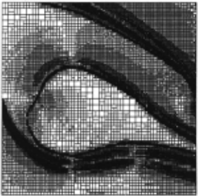
We can combine policy disagreement with the corner­ value difference or value non-linearity criterion in order to take the advantages of both methods : a good approx­ imation of the value function on the whole state-space and an increase of the resolution around the areas of change in the optimal control. We can combine the pre­ vious criteria in several ways, for example by a weighted sum of the respective criteria, or by a logical operation (split if an and/or combination of these criteria is sat­ isfied) . Figure 9 shows the discretization obtained by alternatively, between iterations, using the value non­ linearity criterion and the policy disagreement criterion. We notice that the lower part offrontier 2 is well refined.

3.5 Comparison of the performances

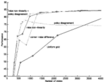
To compare the discretizations, we ran a set (here 256) of trajectories starting from initial states regularly situ­ ated in the state-space, using the policies resulting from the discretizations. The performance of a discretization is defined as the sum of the gain (defined by equation (2)) of these trajectories. Figure 10 shows the respective performances of several splitting criteria as a function of the number of states.

We notice the following points :

• Both the corner-value difference and value non­ linearity splitting processes perform better than the uniform grids . For example, in order to obtain an almost optimal performance of 80, the variable res­ olution grids resulting of these criteria need around four times fewer states than the uniform one.
• The value non-linearity splitting performs slightly better than the corner-value difference one.
• The policy disagreement splitting is very good for a small number of states but does not improve after, and leads to a sub-optimal performance.
• The policy disagreement combined with the value non-linearity gives the best performance.

Can we do better ? So far, we have only consid­ ered local splitting criteria, in the sense that we decide whether or not to split a rectangle according to informa­ tion (value function and policy) relative to the rectangle itself. However, the effect of the splitting is not local : it has an influence on the whole state-space.

4 A global splitting criterion

In the following sections we introduce two new measures of an Markov chain : influence and variance that have been designed to be efficient to provide useful indexes of which parts of state-space are most important to devote data gathering or computational resources to. We derive a global splitting heuristic.

4.1 Influence of a Markov chain

Let us consider a Markov chain whose set of states is 3 = { 6 , .. . , ~n} and probabilities of transition from state ~ to state ~i are p(~; I~). We assume that the discount factor is a function of the state, and is written /r(O with 1 < 1 for some holding timer(~). When the system gets in state~~ it receives a reinforcement R(~) .

We wish to define the influence !(~; I~) of a state ~i on another state ~ as a measure of how much the state ~i "contributes" to the value function of state ~ .

For that purpose, let us define the discounted cumu­ lative k-chained probabilities Pk (~;I~), which represent the sum of the discounted transition probabilities of all sequences of k states from ~ to ~i :

Definition 1 (Influence) Let ~ E 3. We define the influence of a state ~i on the state ~ as the quantity :

Let n be a subset of3. We define the influence of a state ~ion the subset n as I(~;lrl) = L:~EfJ(~;I~) .

We notice that if the holding times r(~) are > 0, then the influence is well defined (and is bounded by 1_ .. /rm;n with Tmin = min~ r(~)). The intuitive idea that I(~i I~) represents the "contribution" of state ~i on the VF of state ~ is formalized by the result that I(~i I~) is the partial derivative of V(~) by R(~;) : I(~; I~)= %~M.).

Moreover , we prove that the influence satisfies the fol­ lowing property :

Computation of the influence. Equation (6) is not a Bellman's equation since the probabilities L:~i p( ~i l~i) do not sum to 1, so we cannot deduce that the successive iterations :

converge to the influence by using the classical contrac­ tion property in max-norm (see [Puterman, 1994]).

However, we have the following property :

Thus, by denoting !(21~) the vector whose compo­ nents are the I(~i 10 and by introducing the 1-norm III(SI~)Ih = 2:::; II(~;I~)I, we deduce that :

and we have the contraction property for the 1-norm which insures convergence of the iterated In(~; I~) to the unique solution (the fixed point) I(~; 10 of (6) .

Illustration on the "Car on the Hill". For a given discretization of the state space, we approximate the optimal control problem by building the correspond­ ing MDP through the process described in section 2.1. Once the MDP is solved, we consider the Markov chain resulting from the choice of the control for the optimal policy u· = 1r*(~) . Let us denote R(~) = R(~, 1r*(~)) , p(~;l~) = p(~;l~, 1r*(~)), and r(~) = r(~, 1r*(~)).

Figure 11 shows (in gray levels) the influence I(~lfl) of the states ~ on n = { 3 points} .

Now define E the subset of states of policy disagree­ ment (in the sense of section 3.3). Figure 12(a) shows E for a regular grid (of 129 x 129). Then, the influence I(~IE) of the states~ onE is plotted in Figure 12(b).

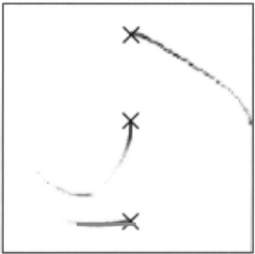
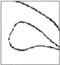
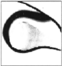
The darkest zones are the places that "contribute" the most to the value function of states in E, thus the areas that are expected to affect the VF at the places of change in the optimal control.

In the following section, we introduce the variance of the Markov chain in order to get an estimation of how accurate the approximation of the VF is, for a given discretization.

4.2 Variance of a Markov chain

By using the notation of the previous section, we have : for any~, V(~) satisfies the Bellman's equation:

which states that V(~)- R(~) is the discounted average of the next values V(~;) weighted by the probabilities of transition p(~i I~). We are interested in computing the variance of these values in order to have an estimation of the range of the values averaged by V(~). We define :

However, the values V(~;) also average some succes­ sive values V(~j), so we would like that the variance also takes into account this averaging, as well as all the follow­ ing ones. In what follows , we define the value function as an averager of the reinforcements and give the definition of the variance of a Markov chain.

The value function as an averager of the rein­ forcements. Let us denote sk(~) a sequence of (k + 1) states (~o = ~,6,6, ... ,~k) whose first one is~· Let Sk(O be the set of all possible sequences sk(~). Let us denote p(sk(~)) = n7=lp(~; l~;-t), the product of the probabilities of transition of the successive states in a sequence, and fori~ k, r;(sk(~)) = z:=~:;;,~ r(~j) the cu­ mulative time of the ith first states of the sequence (with by definition ro(sk(~)) = 0).

We have the property that: z= ·· ({)ES.({)p(sk(~)) = 1. We can prove that the value function satisfies the following equation :

Thus, the value function is expressed as an average of the discounted reinforcements. Now, we can define the variance of these values.

Definition 2 (Variance) We define the variance u 2 (~) of any state ~ E 3 :

We can prove that the limit exists, thus the variance is well defined. Moreover, the variance satisfies :

with e(~) defined by (9). Thus the variance u 2 (~) is the sum of an immediate contribution e(~) that takes into account the variation in the values of the immediate successors ~;, plus the discounted average of the variance u 2 (~;) of these successors.

This is a Bellman equation and it can be solved by DP methods (thanks to a contraction property in max­ norm).

Notice that the variance· defined here has no relation­ ship to the variance of the gain obtained by following any specific policy for the real problem, which is always 0 since the continuous problem is deterministic. Here, the variance indicates the extent of uncertainty on the value function because of the discretization process, and thus gives an estimation of the quality of approximation of the value function for a given discretization.

By using some geometrical considerations (see [Munos and Moore, 1999]), we can prove that e(O is close to 0 in two specific cases : either if the gradient at the iterated point TJ(~, 7!'*(~)) is low (i.e. the values of the successive states ~; are almost constant) or if TJ(~, 7!'*(~)) is close to one corner ~i (then the barycentric coordinate -\{, is close to 1 and the ,\{ 1 (for j f- i) are close to 0). In both of these cases, e(~) is low and implies that the iteration of ~ does not lead to a degradation of the quality of approximation of the value function (the variance does not increase).

Figure 14a shows the standard-deviation u(~) for the Car-on-the-Hill problem for a uniform grid (of 257 by 257). We notice the following points :

• The standard deviation is very high around the dis­ continuity of the value function.
• There is a noticeable positive standard deviation around the 2 frontiers of discontinuity of the gra­ dient of the value function, which correspond to a change in the optimal control. Indeed, in these areas, the VF is the average of the discounted re­ inforcement for different exit times (depending on whether the car can reach the goal directly or has to do one more loop).
• Apart from these areas, the standard deviation is very low, which means that the discounted rein­ forcements averaged by the value function are al­ most constant. A refinement of the resolution in these areas has no chance of producing an zmpor­ tant change in the value function.

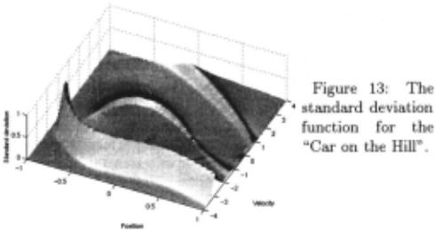
Thus it appears that the areas where a splitting might affect the most the approximation of the value function are the cells whose corners have the highest standard deviations.

4.3 A global splitting heuristic

Now we combine the notions of influence and variance described in the previous sections, in order to define a non-local splitting criterion. We have seen that :

• The states ~ of highest standard deviation u(~) are the states of highest uncertainty on the qual­ ity of approximation of the VF, thus the states that could improve the most their approximation accu­ racy when split (see figure 14(a) for an illustration on the Car-on-the-Hill).
• The states ~ of highest influence (see figure 12(b)) on the set n of states of policy disagreement (figure 12( a)) are the states whose value function affects the area where there is a change in the optimal control.

Thus, in order to improve the precision of approximation at the most relevant areas of the state-space (i.e. where there is a change in the optimal control), an heuristic should be to split the states of highest Stdev_/nfcriterion

(see figure 14) where :

Figure 15 shows the discretization obtained by split­ ting the states of highest Stdev_lnf.

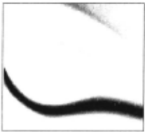
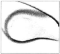
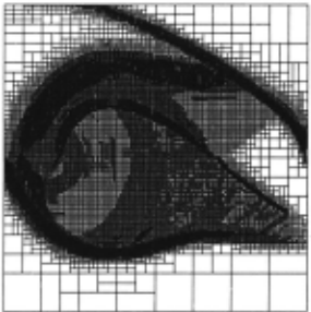
We observe that the Stdev_lnf criterion does not split the areas where the VF is discontinuous unless some re­ finement is necessary to get a better approximation of the optimal control. This turns out to be critical in higher dimensions, where the cost to get an accurate ap­ proximation of the VF is too high.

5 Illustration on other control problems

5.1 The Cart-Pole problem

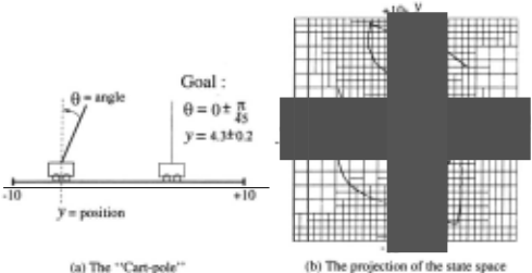
The dynamics of this 4-dimensional physical system (il­ lustrated in figure 16( a)) are described in [Barto et al., 1983]. The goal is defined by the area : y = 4.3 ± 0.2, 8 = 0 ± ; 5 , (and no limits on iJ and 8). This is a much narrower goal than in previous cart-pole RL work. No­ tice that "minimum time maneuver to a small goal re­ gion" from an arbitrary start state is much harder than merely balancing the pole without falling. The current reinforcement is zero everywhere and the terminal rein­ forcement is -1 if the system exits from the state-space, and + 1 if it reaches the goal.

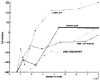
Figure 17 shows the performance obtained for several splitting criteria previously defined. Note that the lo­ cal criteria do not perform better than the uniform grids because the VF is discontinuous at several parts of the state-space (because of boundary problems similar to the frontier 1 of the "Car on the Hill" problem) and the value-based criteria spend too many resources on ap­ proximating these useless areas. But note too that the Stdev_lnf criterion performs very well because it avoids this problem.

5.2 The Acrobat

The Acrobat, which has a 4-d state-space, is a two-link arm with a single actuator at the elbow (see figure 18) . Here, the goal of the controller is to balance the Ac­ robat at its unstable , inverted vertical position, in the minimum time.

This actuator exerts a torque between the links. In [Sutton, 1996b] the goal was to lift the hand to a given height, but here we perform the harder task of balancing the Acrobat at its unstable, inverted vertical position, in the minimum time. The goal is defined by a very narrow range of t 6 on both angles around the vertical position 81 = ~~ 82 = 0 (figure 18(b)), for which the system re­ ceives a reinforcement of R = +1. Anywhere else, the reinforcement is zero. The two first dimensions (81 , 82) of the state space have a structure of a torus (because of the 2rr modulo on the angles), which is implemented in our structure by having the vertices of the 2 first dimen­ sions being angle 0 and 2rr pointing to the same entry for the value function. Figure 19 shows the performance.

Interpretation of the results : As we noticed for

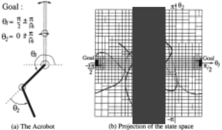
__ Figure 19: Com. ~, ~-~~~-· parison of the performances on the acrobot problem for several splitting criteria.

"0

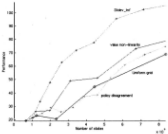
the two previous 4d problems, the local splitting crite­ ria fail to improve the performance of the uniform grids because they spend too many resources on local consid­ erations (either approximating the value function or the optimal policy). For example, on the Cart-Pole prob­ lem, the value non-linearity criterion will concentrate on approximating the VF mostly at parts of the state space where there is already no chance to rebalance the pole. And the areas around the vertical position (low B), which are the most important areas, will not be refined in time (however, if we continue the simulations after about 90000 states, the local criteria start to perform better than the uniform grids, because these areas get eventually refined).

The Stdev_lnf criterion, which takes into account global consideration for the splitting, performs very well for all the problems described above.

6 Conclusion

In this paper we proposed a variable resolution dis­ cretization approach to solve continuous time and space control problems. We described several local splitting criteria, based on the VF or the policy approximation. Local value-based splitting is an efficient, model-based, relative of the Q-learning-based tree splitting criteria used, for example, by [Chapman and Kaelbling, 1991 ; Simons et al. , 1982; McCallum, 1995). But it is only when combined with new measures based on policy and on global considerations (influence and variance) that we are able to get truly effective, near-optimal performance on our control problems. The tree-based state-space partitions in [Moore, 1991; Moore and Atkeson, 1995) were produced by different criteria (of empirical perfor­ mance), and produced far more parsimonious trees, but no attempt was made to minimize cost: merely to find a valid path. Our planned future work includes pruning, in order to include "specific towards general" grouping of areas that have been over-refined, and studying behav­ ior on continuous stochastic systems such as production scheduling.

Acknowledgments.

This research was sponsored by DASSAULT­ AVIATION and CMU.