
Monitoring Piecewise Continuous Behaviors by Refining Semi-Quantative Trackers
Proceedings of the Sixteenth International Joint Conference on Artificial Intelligence. Qualitative Reasoning and Diagnosis. Pages 1080-1085.
© 1999 International Joint Conferences on Artificial Intelligence
Abstract
We present a model-based monitoring method for dynamic systems that exhibit both discrete and continuous behaviors. MIMIC [Dvorak and Kuipers, 1991] uses qualitative and semiquantitative models to monitor dynamic systems even with incomplete knowledge. Recent advances have improved the quality of semi-quantitative behavior predictions, used observations to refine static envelopes around monotonic functions, and provided a semiquantitative system identification method. Using these, we reformulate and extend MIMIC to handle discontinuous changes between models. Each hypothesis being monitored is embodied as a tracker, which uses the observation stream to refine its behavioral predictions, its underlying model, and the time uncertainty of any discontinuous transitions.
- [Bradley and Stolle, 1996] E. Bradley and R. Stolle. Au- tomatic Construction of Accurate Models of Physical Systems. Annals of Mathematics of Artificial Intelli- gence, 17:1-28, 1996.
- [Crawford et al., 1990] J. Crawford, A. Farquhar, and B. Kuipers. QPC: A Compiler from Physical Models into Qualitative Differential Equations. In Proceedings of the National Conference on Artificial Intelligence (AAAI-90}, pages 365-372, Boston, MA, 1990.
- [de Kleer and Williams, 1987] J. de Kleer and B. C. Williams. Diagnosing Multiple Faults. Artificial In- telligence, 32:97-130, 1987.
- [Dvorak and Kuipers, 1991] D. Dvorak and B. Kuipers. Process Monitoring and Diagnosis: A Model-Based Approach. IEEE Expert, 5(3):67-74, June 1991.
- [Haimowitz and Kohane, 1993] I. J. Haimowitz and I. S. Kohane. Automated Trend Detection with Al- ternate Temporal Hypotheses. In Proceedings of the 13th International Joint Conference on Artificial In- telligence, pages 146-151, Chambery, France, August 1993. IJCAI
- [Iwasaki et al., 1995] Y. Iwasaki, A. Farquhar, V. Saraswat, D. Bobrow, and V. Gupta. Modeling Time in Hybrid Systems: How Fast Is "Instantaneous" ? In Proceedings of the Ninth International Workshop on Qualitative Reason- ing, Amsterdam, The Netherlands, 1995. 1086 QUALITATIVE REASONING AND DIAGNOSIS [Kay and Ungar, 1993] IJCAI
- H. Kay and L. H. Ungar. De- riving Monotonic FUnction Envelopes from Observa- tions. In Working Papers from the Seventh Inter- national Workshop on Qualitative Reasoning about Physical Systems (QR-93}, pages 117-123, Orcas Is- land, Washington, 1993.
- [Kay and Ungar, 1999] H. Kay and L. Ungar. Estimat- ing Monotonic FUnctions and Their Bounds using MSQUID. Technical Report TR AI99-280, University of Texas at Austin, 1999.
- [Kay et al., 1999] H. Kay, B. Rinner, and B. Kuipers. Semi-Quantitative System Identification. Technical Report TR AI99-279, University of Texas at Austin, 1999.
- [Kay, 1996] H. Kay. Refining Imprecise Models and Their Behaviors. PhD thesis, University of Texas at Austin, December 1996.
- [Kay, 1998] H. Kay. SQSIM: A Simulator for Imprecise ODE Models. Computers and Chemical Engineering, 23(1):27-46, 1998.
- [Kuipers, 1994] B. Kuipers. Qualitative Reasoning: Modeling and Simulation with Incomplete Knowledge. Artificial Intelligence. MIT Press, 1994.
- [Loiez and Taillibert, 1997] E. Loiez and P. Taillibert. Polynomial Temporal Band Sequences for Analog Di- agnosis. In Proceedings of the Fifteenth International Joint Conference on Artificial Intelligence, pages 474- 479, Nagoya, Japan, August 1997. IJCAI
- Morgan Kaufmann. [Mcllraith et al., 1999]
- S. Mcllraith, G. Biswas, D. Clancy, and V. Gupta. Towards Diagnosing Hy- brid Systems. In Working Notes of the AAAI 1999 Spring Symposium Series: Hybrid Systems and AI, pages 128-135, Stanford, CA, March 1999.
- [Masterman et al., 1998] P. J. Masterman, F . Zhao, and G. Biswas. An Ontology for Transitions in Physi- cal Dynamic Systems. In Proceedings of the Fifteenth National Conference on Artificial Intelligence ( AAAI- 98}, pages 219-224, Madison, USA, July 1998.
- [Ng, 1991] H. T. Ng. Model-Based, Multiple-Fault Diag- nosis of Dynamic, Continuous Physical Devices. IEEE Expert, 6(6):38-43, December 1991.
- [Nishida and Doshita, 1987] T. Nishida and S. Doshita. Reasoning about Discontinuous Change. In Proceed- ings of the Sixth National Conference on Artificial In- telligence, pages 643-648, Seattle, Washington, 1987.
- [Rickel and Porter, 1994] J . Rickel and B. Porter. Auto- mated Modeling for Answering Prediction Questions: Selecting the Time Scale and System Boundary. In Proceedings of the Twelfth National Conference on Ar- tificial Intelligence, pages 1191-1198, Seattle, Wash- ington, 1994.
- Most papers of the Qualitative Reasoning Group at The Uni- versity of Texas at Austin are available from their home page at http: I /vvv . cs. utexas. edu/users/qr. Link
References were extracted automatically from the PDF and may contain errors.
Full text extracted automatically from the PDF; figures, tables and equations may differ. The PDF is the version of record.
1 Introduction
Physical systems are by nature continuous. However it is natural to simplify models by abstracting isolated regions of rapid change to instantaneous discontinuities separating regions of continuous behavior [Iwasaki et al., 1995; Nishida and Doshita, 1987]. Systems which exhibit both continuous and discrete behaviors are called hybrid systems, where a continuous segment of the system's be havior is called a mode of operation and a discontinuous change is called a transition between modes.
Model-based monitoring relies on a comparison be tween the predicted behavior of a model and the ob served behavior of a physical system. Traditional moni toring approaches typically use a single precise model of the physical system. However, even if the system is be having properly, precise parameter values and functional relat.ion~hips are often not known. More importantly, momtormg systems are designed to detect unexpected events or faults, after which knowledge of the system is by definition incomplete. A reliance on precise models leads to overly-specific predictions, sacrificing accuracy
Benjamin Kuipers
Department of Computer Sciences University of Texas at Austin Austin, TX 78712, U.S.A.
kuipers~cs.utexas.edu
and coverage exactly when it is most important for the monitoring system to consider all possible scenarios.
The MIM!C framework [Dvorak and Kuipers, 1991] addresses this need, first by using qualitative and semi quantitative (SQ) models in the QSIM representation [Kuipers, 1994] to express incomplete knowledge with a guarantee that all possible real-valued behaviors are covered; and second, by tracking multiple qualitatively distinct hypotheses in parallel. SQSIM [Kay, 1998] ex tends the semi-quantitative inference power of QSIM by deriving and reasoning wj.th dynamic envelopes guar anteed to bound the real behaviors consistent with an SQ model. SQUID [Kay, 1996; Kay et al., 1999] is a semi-quantitative system identification method based on SQSIM that assimilates a set of observations to an SQ model over a single continuous mode.
Time uncertainty at a mode transition has a partic ularly explosive effect on the uncertainty of predictions from the SQ model after the transition. Therefore, we fo cus our attention first on getting the most out of SQUID based tracking of a continuous mode hypothesis, and ~eco?d, on dete~ting the mode transition and refining Its time uncertamty. In our approach, the monitoring system starts with a coarse description of the physical system and uses the observation stream to refine the be havior prediction, its underlying model, and the time uncertainty of any discontinuous transition. After pre senting the details of our extensio~ and reformulation of MIMIC, we present a non-trivial example and discuss related work.
2 Tracking Piecewise Continuous Behaviors
A tracker embodies a continuous mode hypothesis and c?nfir~s or refutes the hypothesis by unifying its predic tiOns with the observed behavior. When the observations provide sufficient new information, the tracker may be able to refine the imprecision in the underlying model, and thus make more precise predictions in the future.
2.1 SQ System Identification
A tracker is based on SQUID [Kay et al., 1999], which refines an imprecise model (SQDE) by a process called trend matching. Imprecision in the SQDE is represented by numerical intervals bounding possible values of un known parameters, and by static envelopes - functions bounding the possible graphs of unknown monotonic functions.
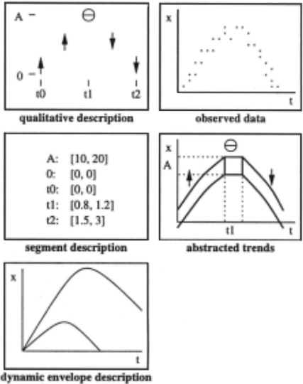
Trend matching compares semi-quantitative trajec tory descriptions derived by SQSIM (the SQ prediction) and the corresponding properties of the observations (the SQ trend) . To refine the underlying model, portions of the model space which cannot plausibly generate the ob servations are excluded.
There are three levels of abstracted properties of the trajectories, corresponding to the level of detail derived by the components of SQSIM: qualitative (QSIM), seg ment (Q2), and dynamic envelope (NSIM) descriptions (Figure 1). The qualitative description is defined by a sequence of symbols(.! .. , 8 and t) representing the deriva tive's sign (qdir) of the trajectory at time points and intervals between time points. The segment description specifies intervals bounding the trajectory at particular time points, i.e., magnitude and time ranges. The dy namic envelope description bounds the trajectory by a lower and an upper envelope. A trend represents the ab stracted properties of the observed data (Figure 1), i.e., symbols representing the qdir, bounding intervals on ex trema and bounding envelopes for monotonic segments.
2.2 Tracker Architecture
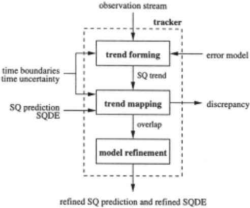
Figure 2 presents the architecture of a tracker. The tracker is initialized with the SQ prediction and the un derlying SQDE of the current mode. Information about the time boundary and the time uncertainty of the cur rent mode may be given. The tracker consumes an ob servation stream and it either produces a refined SQ pre diction and SQDE, or detects a discrepancy between the observation and the prediction. The observation stream is a sequence of samples: numeric values for variables at specified times derived by possibly noisy sensors. Sam ples do not necessarily appear at a constant rate, and need not be synchronized across variables.
Trend forming generates an SQ trend describing each variable in the observation stream by breaking the samples into monotonic segments [Kay et al., 1999). The segments are determined by computing the slope of a linear least-squares fit to the data within a sliding win dow over the samples. Dynamic envelope descriptions for the t and.!.. segments are generated by MSQUID, a neural network-based estimator for monotonic functions [Kay and Ungar, 1993; 1999), out to any given confidence bound. Each e segment is described by the segment's time interval and the minimum and maximum sample values over that interval.
The goal is to detect the qualitative dynamics of the underlying signal in the noisy observation. In the cur rent implementation it is assumed that Gaussian noise of fixed mean and variance is superimposed on the "pure" signal. Each observed variable has an error model that specifies bounds on mean and variance for noise.
Trend mapping compares the SQ trend derived from the observations with the SQ prediction by stepping through both sequences. If an inconsistency is detected between the trend and the prediction, the current hy pothesis is refuted, so the mapping process and the cur rent tracker are aborted.
Qualitative mapping generates a correspondence be tween the qdirs in the SQ prediction and the SQ trend. A successful correspondence may fail to be one-to-one because (i) the samples in the observa tion stream may end before some of the qualitative changes in the SQ prediction take place; (ii) the SQ prediction terminates with a mode change before the end of the current SQ trend, leaving data to correspond to the next mode; or (iii) the SQ predic tion may include small qdir changes which are not detectable in a noisy observation stream.
Segment mapping ensures consistency of corresponding behavior segments in the SQ trend and the SQ pre diction, in the sense that their time and magnitude bounds overlap. Consistency of segments is checked by asserting the segment bounds of the SQ trend to the corresponding segments of the SQ predic tion and propagating these bounds to the other vari ables in the SQDE using Q2's interval propagation [Kuipers, 1994].
Dynamic envelope mapping ensures consistency by in tersecting the dynamic envelopes for corresponding monotonic segments of the trend and the prediction.
Model refinement takes place when trend mapping decreases the bounds on some variables in the SQDE. Parameter imprecision is refined by using Q2 to derive bounds on independent variables from dependent ones. Q2 propagates intervals across model variables at time points and uses the (weak) Mean Value Theorem to propagate those bounds over time intervals. The dy namic envelopes in the SQ trend provide more informa tion than just magnitude and time bounds over mono tonic segments. Model refinement exploits this informa tion by introducing several instantaneous "snapshots" over the monotonic trend segments and propagating the smaller magnitude bounds at these time instants to other model variables. The number of "snapshots" affects the achieved refinement and is specified by the user. F\mc tional imprecision is refined by excluding portions from the static envelopes that are inconsistent with the (re fined) variable bounds. The trend matching techniques guarantee that portions of the model space are ruled out only when they are inconsistent with the observations [Kay et al., 1999].
If a mode change is manifested by a discontinuous change of an observed variable or a sudden sign change of its slope, the change becomes explicit in the purely qual itative trend, and is easy to detect. Otherwise, segment and dynamic envelope trend mapping should eventually refute the current model, but excessive imprecision in the model and uncertainty in the data could prevent the change from being recognized.
Once a mode change has been detected, the tracker for the next mode is initialized with the variable values at the transition point. The new tracker attempts to create a mapping between its SQ prediction and the remaining segments of the observed trend. Time uncertainty in the mode change affects the current tracker and more dramatically the following tracker, in an important way.
3 Refining the Time Uncertainty of Discontinuous Changes
We assume that there are three possible causes for dis continuous changes in the model of a complex system: (i) the autonomous operation of the plant moves from one operating mode to another; (ii) the plant operator takes a known action; and (iii) an unexpected and externally caused event such as a failure takes place. In the first two cases, the current and following modes are known. In the third case, we assume that a separate diagnosis engine proposes a set of fault hypotheses, which MIMIC tracks in parallel. ·
A discontinuous change happens in an instant. Unfor tunately, with imprecise models and noisy and finitely sampled observations, we may never be able to deter mine the precise instant when the change takes place. The best we can do is determine time bounds on the instant when the change occurred.
For matching a piecewise continuous model to a stream of observations, it is particularly important to make the time bounds on discontinuous changes as pre cise as possible. Time uncertainty on a mode change af fects the entire correspondence between prediction and observation in the following mode, resulting in propa gating uncertainty. Figure 6(c) shows how weak time bounds on a discontinuous change can result in ex tremely weak bounds on the prediction of the follow ing mode. Therefore, we focus on improving these time bounds.
3.1 Intersecting Trend and Prediction
We focus here on refining time uncertainty of a mode change based on the intersection of SQ trend and SQ prediction. After semi-quantitative reasoning has pro vided bounds on the transition time, advanced filtering techniques based on statistical or digital signal process ing may be applicable.
When there is time uncertainty, the mapping between the SQ trend and the SQ prediction is not fixed. The SQ prediction can be shifted relative to the SQ trend by any offset within the range of the time uncertainty.
However, a mapping is only valid if the SQ trend seg ment and the SQ prediction segment have a non-empty intersection for every time-point t in the SQ trend. This is exploited to derive refined bounds on the time uncer tainty of discontinuous changes (Figure 3} .
Fort segments, the mapping is valid as long as (i) the upper envelope of the trend is above the lower envelope of the prediction and (ii) the lower envelope of the trend is below the upper envelope of the prediction. More for mally, we can determine the lower bound tcmin and the upper bound tcmax, respectively, as follows:
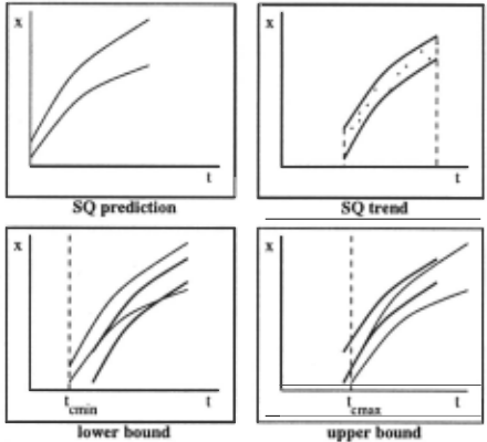
where Xtr(t) is the observed trend for x(t), Xpr(t- t 8 ) is the prediction, shifted by t8 · Over- and under-bars rep resent the upper and lower dynamic envelopes, respec tively. Similar conditions hold for .!. and 8 segments.
This intersection process is applied to all segments of the mode. Improvements in time uncertainty propagate from segment to segment by interval arithmetic and in tersection of bounding intervals.
3.2 Incremental Refinement
When there is a great deal of time uncertainty about the transition from one mode to another, many samples in the observation stream fall within the uncertainty inter val, and thus cannot be unambiguously assigned to one of the adjacent segments of monotonic change. After time uncertainty is decreased, some samples can now be assigned to a definite adjacent segment. The additional information helps refine the mode the segment belongs to, and its underlying model. Improvements to the ad jacent modes can, in turn, lead to further decreases in time uncertainty of the transition. And so on until no further improvement results.
The algorithm for incremental refinement of the time uncertainty between two adjacent modes i and j is pre sented in Figure 4. The trend/prediction intersection (line 7) is performed for each behavior in the succeeding mode. If the trend is inconsistent with the behavior at the qualitative level or no valid mapping can be found for any time offset within the time uncertainty the behavior is refuted (line 9). Since each behavior is independently intersected with the trend this method results in different refinements on the uncertainty interval for each behavior of the succeeding mode.
1 refine-transition(tu, modei, modej, SQtrend) 2 behs +- generate-behaviors(modej) 3 for each behavior beh in behs do 4 t +- tu 5 repeat 6 refine +- false 7 tn +- intersect(beh, SQtrend) 8 if (tn = 0) then 9 refute beh 10 elseif ( tn < t) then 11 t +- tn 12 refine +- true 13 re-assign samples to modei and modej 14 re-track modei 15 inherit refinements from modei to beh 16 endif 17 until not(refine) 18 endfor4 Overall Monitoring System
The overall monitoring system tracks multiple hypothe ses in parallel. The hypotheses may represent different nominal or fault models of the plant, or they may repre sent different qualitative behaviors predicted from semi quantitative simulation of a particular model.
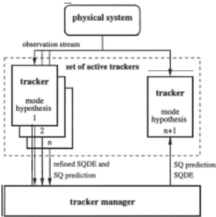
A particular hypothesis is a sequence of mode hy potheses [H1 (to, t1); H2(t1, t2); · · ·; Hn(tn-1, tn)]. The monitoring system alternates between tracking a partic ular mode hypothesis H,(t,_1 , t,) and refining the time uncertainty of the mode transition at ti. Several track ers and their hypotheses may be refined in parallel (Fig ure 5). The achieved refinements (SQ prediction and SQDE) are passed to the tracker manager which instanti ates new trackers and refines the time uncertainty of the mode transition. As discussed in Section 3, we assume that the models for new modes are known. Information from the observation stream, such as the satisfaction of a condition that autonomously moves the system to an other mode or a signal indicating an operator action, allows the tracker manager to choose the model(s) for the new mode. Fault models may also be proposed at any time by a separate diagnosis engine.
Model refinements such as improved variable bounds or static envelopes may be inherited from one model H1 to the next Hi+l across a mode transition. In the cur rent implementation, the user specifies the variables and functional relations whose refinements can be inherited.
The degree of model precision is important for the fault detection performance of our monitoring system. However, with imprecise models, uncertain observation and limited observability we may never be able to detect all faults or distinguish between every possible hypoth esis. In order to achieve a sufficiently precise prediction for fault detection, (i) our initial knowledge about the system must be precise enough or (ii) we must collect enough data from the "healthy" physical system to re fine its model to the required degree of precision.
5 Experimental Results
We demonstrate the refinement capabilities of our mon itoring system using a two tank system. In this example (Figure 6(a)), we start with a filled upper tank and an empty lower tank; the drains of both tanks are open and the upper tank is filled at a constant inflow rate. When the amount in the upper tank drops below a limit the in flow rate is increased. This scenario is modeled as a tran sition between two operating modes (Figure 6(b)) . Only imprecise information is known about this scenario, i.e., intervals for variables and bounding envelopes for func tional relations. Since both tanks remain unchanged, the refinements of the variables a and b as well as of the functional relations f and g are inherited from the first to the second mode.
SQSIM predicts 9 different behaviors for the two tank scenario; 5 of them include the region transition. Only one is consistent with the SQ trend; the other trackers are refuted. Figure 6(c) shows the predicted dynamic envelopes for the amount in the lower tank for the sur viving prediction. SQSIM predicts the time of the mode transition as (1.68, inf] .
The observations are generated by numeric simulation of an ODE, adding Gaussian noise with fixed mean and variance to the samples. The exact model for deriving t~e samples is given as a' =if a- 9Ja, b' = 9Ja- 8Vb with a(to) = 95, b(t0 ) = 0, c = 9 and an inflow rate ifa = 25 before and ifa = 60 after the transition. The samples are generated at a rate of 20 Hz.
Figure 6(d) shows the samples and bounding envelopes derived by trend forming for the variable b. MSQUID
| obs. vars. | a(t) | b(t) | I | g | tc |
|---|---|---|---|---|---|
| none | 1 | 1 | 1 | 1 | 1.68, inf] |
| b | 1 | 0.53 | 1 | 1 | 2.70, 4.20 |
| a,b | 0.29 | 0.22 | 0.68 | 1 | 3.73, 4.14 |
| a,b,ofa,ofb | 0.26 | 0.18 | 0.28 | 0.40 | 3.78, 4.14 |
| obs. vars. | a(t) | b\.tT | f | g | tc |
|---|---|---|---|---|---|
| b | 1 | 0.70 | 1 | 1 | 2.50, 4.25 |
| a,b | 0.64 | 0.56 | 0.96 | 1 | 2.87, 4.25 |
| a,b,ofa,ofb | 0.61 | 0.47 | 0.57 | 0.58 | 2.98, 4.25 |
constructs the bounding envelopes around the observa tions to achieve a certainty of 95%. This figure also presents the final refinement achieved by the monitor ing system. The dynamic envelopes for b are refined to 18% of their initial area and the time uncertainty is refined to (3.78,4.14) after two iterations of the re finement algorithm 1 . Observations for a, b, of a and ofb, with noise J.L = 0 and var = 1, are used in this case. ~ote the propa?ation of refinements through the SQDE, 1.e., the dynamic envelopes in the first segment are nar rower than the bounding envelopes of the observation of b. Due to time uncertainty, the dynamic envelopes in the second mode are wider than the bounding envelopes of the observation.
The effect of observability is shown in Table 1. This table presents the achieved refinements dependent on the observed variables. The degree of refinement is defined by the ratio of the predicted and refined areas for vari ables and functional relations. For the variables a and b the area is specified by the dynamic envelopes over th~ observation time. For the functional relations f and g, the area is specified by the bounding functions (static envelopes) over the range of f and g. The achieved re finement of the time uncertainty is represented by tc . As the number of observed variables increases the re finement improves and extends to more variables and functional relations. Table 2 presents the reduced refine ments caused by an increase of noise in the observation.
6 Conclusion
We have presented a method for monitoring dynamic systems that exhibit both discrete and continuous be haviors. The monitoring system refines the behavior pre diction, the underlying model and the time uncertainty of discontinuous changes. The hypothesis is refuted and pruned from the tracking set when refinement eliminates all possible values for any parameter.
Trend matching uses a statistical best fit to observed
1 1n our experiments incremental refinement never required more than 3 iterations; it usually stopped after 1 or 2.
,---------------1
(b) Imprecise model with mode transition
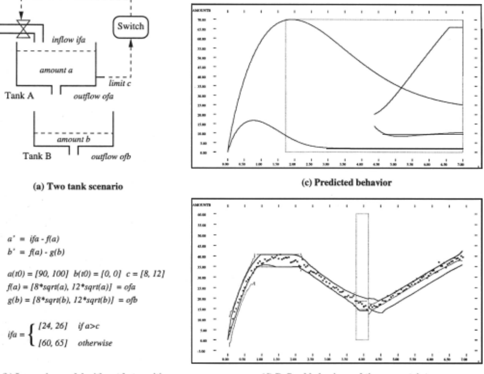
Figure 6: A two tank scenario (a), modeled as an autonomous mode transition (b), its prediction (c) of the upper and lower bounds (dynamic envelopes) forb, and the refined bounds and time uncertainty (d). In both graphs, the solid lines represent the predicted or refined dynamic envelopes. The dotted box represents the time uncertainty of the mode change; the dashed lines represent the bounding envelopes of the observations (d). Due to the time uncertainty of the discontinuous change the prediction of the second mode can start at any time within the dashed box. For the sake of readability, they start in the middle (c) and at the right end (d) of the dashed box, respectively.
data, plus bounding envelopes out to any desired confi dence bound. Portions of the model space are removed only when they are inconsistent with these bounds. This gives a good (and adjustable) compromise between ag gressiveness and robustness in handling noise and unin formative data.
Related work has been done by [Masterman et al., 1998). In their framework for model-based diagnosis the physical system is modeled by a temporal causal graph. Qualitative candidate models are derived from this representation and parameter estimation techniques are applied to fit the candidate models to the obser vation. TrenDx [Haimowitz and Kahane, 1993) is a monitoring system which uses a semi-quantitative rep resentation of a behavior and attempts to fit data to this behavior representation. Since TrenDx uses predefined behavior templates no refinement can be per formed. PRET [Bradley and Stolle, 1996) automatically constructs a precise ODE model of a physical system. PRET focuses on system identification and not on mon itoring. Loiez and Taillibert [Loiez and Taillibert, 1997) use piecewise polynomial functions, so-called temporal band sequences, to bound the observation stream. The behavior of components in analog circuits is modeled by sums of temporal functions including derivatives of any order. This approach is only able to detect discrepancies but not to predict the behavior of the system. Mcllraith et al. [Mcllraith et al., 1999) present an approach for diagnosing hybrid systems where all mode transitions, i.e., the history of executed actions, are known. Can didate generation and model estimation are based on the model-based diagnosis framework of [Masterman et al., 1998] and the tracker framework is adopted to refine multiple candidates.
FUrthermore, our monitoring method is directly ap plicable to fault diagnosis in dynamic systems. Fault hypotheses can be proposed for monitoring based on initial weak information such as the signs of discrep ancies between observations and predictions, by using existing methods such as [de Kleer and Williams, 1987; Ng, 1991]. Automatic model-building methods can select relevant model-fragments from a background knowledge base to express initially weak knowledge about a fault as an SQDE [Crawford et al., 1990; Rickel and Porter, 1994]. The observation stream is then used to refine or refute each proposed model.
Acknowledgments
This work has taken place in the Qualitative Reason ing Group at the Artificial Intelligence Laboratory, The University of Texas at Austin. Research of the Qual itative Reasoning Group is supported in part by NSF grants IRI-9504138 and CDA 9617327, by NASA grants NCC 2-760, NAG 2-994 and 9-898, and by the Texas Ad vanced Research Program under grants no. 003658-242 and 003658-347. Bernhard Rinner is supported by the Austrian Science FUnd under grant number J1429-MAT.
@inproceedings{ijcai1999p154,
  title     = {Monitoring Piecewise Continuous Behaviors by Refining Semi-Quantative Trackers},
  author    = {Rinner, Bernhard and Kuipers, Benjamin},
  booktitle = {Proceedings of the Sixteenth International Joint Conference on
               Artificial Intelligence, {IJCAI-99}},
  publisher = {International Joint Conferences on Artificial Intelligence},
  editor    = {Thomas Dean},
  pages     = {1080--1085},
  year      = {1999},
  note      = {Qualitative Reasoning and Diagnosis},
  url       = {https://ijcai.org/proceedings/1999/154},
}
TY - CPAPER TI - Monitoring Piecewise Continuous Behaviors by Refining Semi-Quantative Trackers AU - Rinner, Bernhard AU - Kuipers, Benjamin T2 - Proceedings of the Sixteenth International Joint Conference on Artificial Intelligence, IJCAI-99 PB - International Joint Conferences on Artificial Intelligence PY - 1999 SP - 1080 EP - 1085 UR - https://ijcai.org/proceedings/1999/154 ER -Copied
Machine-readable versions of this paper, for tools and AI agents:





