Modeling Time in Hybrid Systems: How Fast Is "Instantaneous"?

1 Introduction

Many of today's electro-mechanical devices exhibit both continuous and discrete behavior. Modeling these hybrid systems presents special challenges for automated mod­ eling and simulation. Work in discrete event simulation [Cassandras, 1993] assumes that all change is discrete; work in quantitative and qualitative simulation assumes that all change is (at least piecewise) continuous. The behavior of hybrid systems, such as digitally controlled copiers, chemical plants , automobiles, and so on, is not appropriately characterized as either continuous or dis­ crete.

A hybrid model of a system is often the result of an abstraction that simplifies analysis and the prediction of behavior. For example, we often view closing a switch as causing the voltage difference across the switch to be­ come 0 in an instant ; a level sensor in a reactor vessel causes a pump to shut off and a valve to close in an instant. In principle, it is possible to construct continu­ ous models of these behaviors, but they are considerably more complicated. In practice, the use of discontinu­ ous abstractions is both ubiquitous and necessary. For instance, the transient behavior of control electronics is often irrelevant to the task of analyzing the overall sys­ tem. Complex sequences of discrete actions are also pos­ sible, such as when an automobile ignition is turned on (relative to the vehicle's motion) or a camera's shutter is depressed.

A satisfactory model for hybrid systems must support :

• discrete actions occurring in the presence of contin­ uous change;

Vijay Saraswat, Daniel Bobrow, Vineet Gupta

Palo Alto Research Center XEROX Corporation 3333 Coyote Road Palo Alto, CA, 94304

• complex sequences of discrete actions;
• the abstraction that discrete actions are instanta­ neous.

We can refine the third criterion: it must not be possi­ ble to measure the duration of a discrete action with a continuous real-valued clock.

There have been several attempts to introduce dis­ crete changes into a continuous model [Forbus, 1989; Nishida and Doshita, 1987; Iwasaki and Low, 1992). Problems with the mathematical semantics arise, how­ ever, because discrete changes violate the assumption of continuity. Giving sound semantics to the representation of discrete changes while employing the real number line as the model of time (as is usually employed in model­ ing of continuous systems) and respecting the underlying semantics of continuous change turns out to be very dif­ ficult .

We provide a sound mathematical basis for modeling hybrid systems that satisfies the three desiderata listed above. The hybrid systems are specified by discrete ac­ tions as well as qualitative or quantitative continuous functions . Our solution is based on nonstandard analy­ sis [Hoskins, 1990]. We employ a nonstandard model of time, which captures the intuitive distinction we would like to make between discrete and continuous changes. More importantly, it allows us to model both continuous and discrete changes uniformly without contradictions or introducing unnecessary complexity.

2 Discrete Actions in Continuous Systems

Consider the simple circuit shown in Figure 1, in which electric power is provided to a load either by a solar ar­ ray or a rechargeable battery. The charge on the battery is maintained by a solar array. When the charge level of the battery exceeds a threshold, the charge-current con­ troller opens the relay, allowing the battery to provide power to the load. When the charge level drops below another threshold, the charge-current controller closes the relay, allowing the solar array to recharge the bat­ tery. It is natural to model this system by a mixture of continuous and discrete behavior.

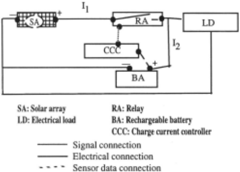
The following axioms define the continuous behavior of the system. A continuous change is specified by a form C : c => e, where C is the name of the continuous change, c is the condition for the change to take place, and e is its consequences. The antecedents, c, and the consequences, e, hold simultaneously. We will use the notation c(t) to denote that c holds at timet .

• CO: shining(sun) 1\ closed(relay) =>It =it When the sun is shining and the relay is closed, the solar array acts as a constant current source.
• Cl: closed(relay) =>It+ h = 0 When the relay is closed, it acts as a simple conduc­ tor.
• C2: "'closed(relay) => It = !2 = 0 When the relay is open, it conducts no current.
• C3: -h = d~fA The battery accumulates charge.

Likewise, the following axioms define the discrete be­ haviors of the relay and controller. A discrete behavior is specified by a form D : c---+ e, where D is the name of the discrete change, c is the condition for the change to take place, and e is its effect.

• Dl: high(signal) 1\ closed(relay)--> "'closed(relay) When the signal from the controller goes high, the relay opens.
• D2: "'high(signal) 1\ "'closed(relay) ---+ closed(relay) When the signal from the controller goes low, the relay closes.
• D3: QBA 2: Q2/\ "'high(signal)---+ high(signal) When the controller detects the charge level in the battery has reached q2, it turns on the signal to the relay.

Since each one of Dl - D3 represents an actual ac­ tion of a physical component, it does take some non­ zero amount of time for the consequences to take ef­ fect after the condition becomes true. However, the dis­ crete actions are extremely fast relative to the contin­ uous changes, and their dynamics are uninteresting for the purposes of modeling the overall circuit. Thus, we would like to model them as being instantaneous. In other words, we would like the model to capture the no­ tion of almost instantaneous change taking place without any measurable duration.

While intuitively plausible, this interpretation of in­ stantaneous changes raises a fundamental problem in modeling of continuous systems. Typically, time is taken to be isomorphic to the real number line. Thus, any tem­ poral behavior can be viewed as a sequence of states that hold alternately at an instant and over an open interval (this representation is also used in qualitative reasoning). It works very well when there are no discrete changes. The qualitative behavior of the system, without the dis­ crete behaviors specified by Dl through D3 , is shown in Figure 2(a) . In the portion of the behavior shown in Figure 2, QBA is steadily increasing, until it reaches the threshold q2 at time t = t2. States sa and s2 are instantaneous states at tiine points t0 and t 2 ; St and s3 are states corresponding to the open intervals (tt t2) and (t2 + oo).

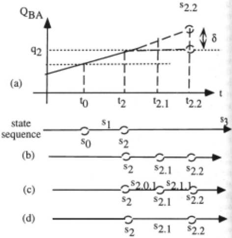
Add to this behavior the actions of the controller and the relay represented by the actions Dl-D3. The an­ tecedent of D3 becomes true in the instantaneous state s2 . Thus, at the time t2.t , immediately following t2, the signal goes high. At yet another time (t2.2) immediately following ht, the relay opens due to action Dl. Our in­ tuitive notion about these instantaneous changes is that they happen so fast that the values of continuous vari­ ables do not measurably change during the short time required for the consequence of an action to take effect. This intended sequence of states are shown in Figure 2(b) . The contents of the states are summarized below.

• s2 at time t2: QBA q2 1\ closed(relay) 1\ ""high( signal)

The antecedent of D3 holds, which makes the con­ troller turn on the signal to the relay.

• s2.1 at time t2.1: high(signal) 1\ closed(relay) The consequence of D3 holds; the antecedent of D1 holds , which makes the relay start to open.
• s2.2 at time t2.2: ""closed(relay) The consequence of D1 holds.

If we use the real number line as the model of time, it is impossible to produce a description that matches exactly our intended interpretation of the discrete actions. On the real number line, there is no well-defined notion of a point immediately following a point . Even though we would like to say that there is a time point at which Signal goes high and which "immediately follows" t2, we cannot because the point t 2 must be followed by an open interval of non-zero length. This forces us to take one of the following approaches:

1. Since actions are supposed to take little time, as­ sume that they take no time . In other words, rules such as D1 through D3 are treated just like ordinary logical implications with respect to time.
2. Always insert a small, open interval of unspeci­ fied length between the time points at which conse­ quences of actions become true. This corresponds to the state sequence in Figure 2( c). States s2.o .1 and s2 .1.1 last over small open intervals.
3. Make the consequences of an action true in either the point or the interval· that immediately follows the current state. This corresponds to the state se­ quence in Figure 2(d). States s2 and s2 .2 are instan­ taneous while s2.1 lasts over a small open interval.

Each of these approaches has difficulties. Approach 1 is obviously flawed - if actions are logical implications, then any of D1-D3 directly produces a contradiction. In general, there are many control actions that take place only if the desired effect is not already in place. The an­ tecedent for such actions will include the negation of the consequence; this immediately leads to a contradiction when actions are treated as implications.

With both approaches 2 and 3, the value of "continu­ ous" variables become unknown after a sequence of ac­ tions. There are two possibilities for the value of Q8 A at time h2 as shown in Figure 2(a). Since the sun remains up and the relay remains closed until state s2.2 , QBA continues to increase past q2 until s2.2 . Since there is a non-zero amount of time that passes between s2 and s2.2, QBA must have some value above q2, say q2+8, where 8 is some positive quantity of unknown magnitude. As sim­ ulation continues and other discrete actions take place, variables can accumulate a number of such unknown 8's, unnecessarily complicating value computation.

If we ignore such 8's (since actions happen so fast that any change in the values of other continuous vari­ ables over the time is negligible), we introduce a con­ tradiction. In the above example, if we assert that QBA(s2) = QBA(s2.2) = q2, it will be inconsistent with the basic assumption that QBA is a continuous quantity and the fact that, in the given situation, the condition of C3 holds and therefore QBA should be continuously increasing over the interval between s2 and s2.2·

Option 3 has the additional disadvantage of arbitrarily assigning an instant or an open interval to the duration of an action depending on where it happens to appear in a sequence. If the first action in a sequence occurs at a time instant , then all odd-numbered actions will occur at an instant. If it had occurred over an interval, then all odd-numbered actions would occur at intervals. This is an undesirable and bizarre artifact of the particular model of time employed and has nothing to do with what the actions represent .

This example has demonstrated problems that arise when we try to represent hybrid systems while using the real number line as the model of time. In summary, the problems are

1. We cannot have a sequence of instantaneous states one immediately following the other.
2. We cannot ignore the change, if any, in the value of continuous variables over the time in which discrete actions take place.

We propose to use the hyperreals as our model of time. This allows us to represent discrete actions in a natural way and to overcome these two problems.

3 Calculus of Hyperreals

This section briefly reviews the fundamental concepts in nonstandard analysis that are relevant to our approach.

The calculus of hyperreals is defined over the set * R, such that * R is a totally ordered field and contains R as its proper subfield. The members of R are called standard members of* R. Nonstandard members of* R include infinite and infinitesimal numbers. The elements of * R can be generally classified as follows:

• An element w of * R is called an infinite hyperreal number if Va E R, w >a. We will denote the set of all infinite hyperreal numbers as *Roo.
• An element t. of* R is called an infinitesimal hyper­ real number if Va E R, lei ::; Ia!. We will denote the set of all infinitesimal hyperreal numbers as * R0 · Note 0 is the only standard member of* R0 .
• An element b of* R is called a finite hyperreal num­ ber if there is a positive number a E R, such that lbl ::; a . We will denote the set of all finite hyperreal numbers as* RJ· Note* RoC * RJ.

We will use lowercase alphabet letters to denote a member of · R1 , t: with or without a subscript to denote a member of · Ro, and w with or without a subscript to denote a member of · Roo.

The standard arithmetic operators are defined over · R in an intuitive manner. The following axioms follow from their definitions.

The value of w *t: can be a member of · Rj, · Roo, or · R0 . We will also use the notation ~ to mean "infinitely close" defined as follows:

The following theorem holds:

Theorem 3.2: Each member of · R1 is infinitely close to a unique member of R.

In other words, Va E *R1 , 31' E R such that a = r + c and r is unique. We will call such r the standard part of a and denote it as 0 a.

Corollary 3.3: Each interval of an infinitesimal length contains at most one element of R. Some examples are (t- t:, t + t:), (t:, 2t:), and (w, w + t:).

In summary, a system · R of hyperreal numbers is R extended with infinite numbers of infinitesimal and infi­ nite elements, and it is closed under addition and mul­ tiplication. A significant aspect of · R for our present purpose is that it gives us the notion of infinitesimal dif­ ferences between two points of time (or quantity values) that are smaller than the difference between any two standard real numbers. Furthermore, infinitesimal dif­ ferences never add up to a standard number as long as there are only a finite number of them.

In order to make · R our model of time (and the range of continuous functions), we must have a definition of continuity in · R. In standard analysis, continuity of a function f at a is defined as

In nonstandard analysis, continuity1 of a function · f is defined in an analogous manner as:

Definition 3.5: · f is Q-continuous at a in · R iff Vx[x ~a:::} · f(x) ~ · f(a)].

The derivative · f' of · f at a is defined as follows:

Definition 3.6: If Et, t:2 # 0 and Et, t:2 E* Ro,

and

In other words, the derivative is defined to be a stan­ dard number and the derivative is constant in the vicin­ ity(a-t:, a+t:)ofa.

1 There are actually several different notions of continuity that can be defined in · R. Q-continuity is one of them.

4 A Nonstandard Model of Hybrid Systems

We now describe our model of hybrid systems based on calculus of hyperreals and show how our approach over­ comes the difficulties discussed in Section 2.

We use the hyperreals as the model of time as well as of the domain of continuous functions. We assume that the functions used to describe the continuous part of the behavior are Q-continuous in · R. Discrete actions are understood as follows: D : c -+ e means that whenever c holds at to, there is a t 1 > to such that to ~ t 1 and e(t1). A more precise semantics is given in Section 5.

This definition of an action allows us to have a se­ quence of instantaneous states one after another, each of which is distinct but infinitely close to its predecessor. Furthermore, the value of a continuously changing vari­ able changes only by an infinitesimal magnitude over any finite sequence of such instantaneous states. Therefore, if we want to compute the standard part of a continu­ ously changing variable's value, we can always ignore the nonstandard part when the number of discrete changes is finite . The nonstandard part can never become large enough to make a difference in the standard part.

Note that forD : c-+ e, we do not require that e entail ·c (as is the case in all the examples of discrete actions in Section 2). However, it is in general a good idea to represent actions in such a way that the consequence invalidates the condition because, otherwise the action will end up being repeated an infinite number of times.

The example in Figure 1 yields a state sequence as depicted in Figure 3, where the time axis is now the hy­ perreal number line. The states 82, 82.1, and 82.2 are distinct states, but the gaps between them are infinites­ imal. Thus, we can safely say that the standard part of the value of QBA in state 82.2 is equal to that in state s2 without contradicting the continuity assumption or the equation in C3.

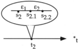
Notice that this semantics of continuous and discrete behavior based on nonstandard model of time allows us to capture in the most natural way what we mean in­ tuitively by discrete actions without violating the basic continuity assumptions. It also allows us to avoid in­ troducing b's of an unknown magnitude into the value of continuously changing variables, unnecessarily complicating computation.

4.1 Temporal Projection

The task of modeling hybrid systems requires both a mathematical foundation that allows the behavior of a hybrid systems to be described and algorithms that pre­ dict the behavior from such a description. In this section, we discuss the problem of prediction, particularly with regard to predicting behavior across discrete changes.

Predicting behavior requires us to solve the "temporal projection" problem. During phases of continuous be­ havior, temporal projection is straightforwardly solved by differential calculus. The equations describing a sys­ tem together with the values of variables can be solved to determine future behavior. Difficulties may arise when a discrete action occurs - a single discrete change may cascade through equations and other constraints, result­ ing in discontinuities in the values of many other contin­ uous quantities. For example, dumping hot water into a container holding some cold water results in discontinu­ ous changes in the mass of water, its level, temperature, pressure at the bottom, and so on. It does not, how­ ever, change the specific heat of the water, the location of the pot, its color, and so on. In the circuit of Figure 1, opening the relay may cause discontinuous changes in the values of the current and voltage at various points in the circuit, but not in the charge level of the battery.

What we are faced with is a special case of the prob­ lem of retaining predications across an action, which has been widely studied in the AI literature. There are two basic approaches: either explicit frame axioms are re­ quired to carry predications across discrete changes (e.g., STRIPS [Fikes and Nilsson, 1971]), or the logic is ex­ tended with some sort of accessibility relation and pref­ erence relation between possible worlds (e.g., Action­ Augmented Envisionment [Forbus, 1989] or any of the non-monotonic logics for expressing action). Unfortu­ nately, neither approach is altogether satisfactory. Pro­ viding explicit frame axioms is error-prone and difficult because the frame axioms cannot be specified for indi­ vidual actions or predicates in isolation. Providing an accessibility and preference relation that eliminates im­ plausible consequences (but not plausible ones) while be­ ing computationally tractable remains elusive. Further­ more, as Forbus points out in [Forbus, 1989], there is no formal standard for correctness here; there are only informal desiderata. The primary one is that changes should be minimal and causally related to the action. In the case of predicting behavior of hybrid systems, combi­ nations of the two approaches appear to be quite promis­ ing.

The Device Modeling Environment (DME) [Iwasaki and Low, 1992] combines explicit frame axioms with a preference relation. DME uses an algorithm for tem­ poral projection over discrete changes that appears rea­ sonably efficiently and avoids implausible consequences. DME is a modeling and simulation program for hybrid systems where continuous changes are described by a set of algebraic and ordinary time differential equations and discrete changes are described by actions as discussed throughout this paper. When a discrete change takes place, DME prefers among all the states that can result from the action those states that satisfy the following criteria:

1. The consequence of the action is true in the state.
2. The values of a variable that is exogenous, inte­ grated, or discrete remains the same unless the vari­ able is explicitly changed by the action.
3. The values of the variables that are specified not to change across discrete changes in user-provided, domain-specific frame axioms remain the same.

Integrated variables are those quantities whose val­ ues at time t is the integration of changes up to that time; unless changed explicitly, their values should not change instantaneously. Likewise, exogenous variables are those controlled by entities external to the model; unless changed explicitly, their values are not likely to change. Finally, since DME assumes that all mecha­ nisms for change (continuous or discrete) are represented as equations or actions, and continuous equations cannot change the value of a discrete variable, the value of such a variable is likely to remain the same unless changed explicitly by an action.

Based on the projected variable values, DME deter­ mines what equations should be in effect and recomputes the values of all other variables using the equations. This may or may not result in discrete changes in the values of recomputed variables. If there is not enough informa­ tion to complete the state description after projecting values from the previous state, the behavior prediction will branch and DME will produce all possible successor states. DME also allows the user to specify explicitly what quantities can be projected over discrete changes, since the user or the model builder often has knowledge that allows her to provide such domain-specific frame axioms a priori. This strategy avoids producing incon­ sistencies by being conservative about value projection while allowing improved efficiency when domain-specific frame axioms are available.

5 A Logic for Hybrid Systems

Section 4 has defined a model of hybrid systems based on nonstandard analysis that satisfies the desiderata out­ lined in the introduction. This model may be employed in several ways. It may be embedded into first order logic. A common method for representing actions and change in first order logic is to take time-varying pred­ icates and augment them with an additional argument that ranges over the times that the predicate holds. This argument may be allowed to range over the hyperreals instead of the reals. If the mathematical definitions of continuity, etc., over the hyperreals are added, then one can reason about the behavior of systems so described. It is often desirable, however, to construct a slightly re­ stricted logic that will enforce the common idioms and allow them to be more succinctly expressed. For ex­ ample, temporal logics typically prevent explicit refer­ ence to and quantification over time, as well as making temporal statements much more succinct. It is possible to define a temporal logic similar to Henzinger's Hibrid Temporal Logic [Alur et al., 1993], and replace the real line with hyperreals. We will pursue yet another possibil­ ity here and construct a logic specifically for the purpose of predicting and analyzing the behavior of hybrid sys­ tems. The key idea is that the denotation of sentences will be given by possible temporal behaviors where time can take on hyperreal values.

Our logic is based on the approach of concurrent con­ straint programming [Saraswat, 1993] . Concurrent con­ straint programming uses the idea of a store as the set of possible values of the variables. Programs can then add constraints to the store, and ask the store if some constraints are valid.

Our language modifies the standard concurrent con­ straint languages, which are atemporal, by allowing the language constructs to extend across time. Thus, the store also varies over time. The language is built over a constraint system, and we assume that the constraint system is powerful enough to express the desired prop­ erties. In particular, the constraint system can express differential equations and propositional logic.

The syntax of the language is:

c represents the constraint being added to the store. We will assume that it stays there until a discrete action adds its negation to the store. D : c =>A is used to represent simultaneous actions, for example those in Figure 2 (D is the name of the constraint). D : c -+, A represents a discrete action, so A holds an f time after c becomes true. 2 (A, B) is used to put together several such con­ structs to form a program. first cis used to specify that c is true at the start of an interval.

The model we have for these programs is a set of func­ tions from the hyperreals to sets of constraints. Each such function represents a possible evolution of a pro­ gram, describing the constraints that are present in the store at any time instant. The only restriction that we place on these sets of functions is that they be deter­ minate. That is, for any evolution o up to time t, the set {!( t) I f extends o} is closed under greatest lower bounds. 3 This enables us to determine uniquely the out­ put of a process given as a set of functions .

The denotation of a program P in our language, writ­ ten [P] , is the set of all of its possible evolutions. We can define the denotation compositionally as follows. [ c] is the set of all functions where f(t) ;:2 c until some t when f(t) ;:2 · c. [c => A] is the set of all functions in which whenever c is true at timet, then the function starting at t is in [A]. [c -+, A] contains those functions f in which whenever c is true at t, then f starting at t + f is in [A]. Notice that in order to get determinacy, we need to know a fixed <, and also since f is an infinitesimal, we need hyperreal functions here. [A, B] = [A] n [B]. This last definition provides the motivation for including all of the functions f(t) ;:2 c, rather than something like f(t) = c. Including the supersets allows composition to be defined as intersection.

2 The construct D : c -+ A used in Section 2 can be thought of as D : c -+, 0 A, for some fixed co.

3 f extends o if f(x) = o(x) for all x < t , where o is defined up to t .

As an example, consider the following program:

For any function f in its denotation, we must have

• f(O) ;:2 {x' = 1, x = 0, (Power On)} ,
• /(3) ;:2 { x' = 1, (Power On)},
• /(3 + cl) ;:2 {x' = 1, (Power On) , (Relay Open)},

and so on. This gives us all the information we need about the process, and we can use it to deduce various things as shown below.

Once we have a denotational model for our programs, we immediately get a logic for the language. Given pro­ grams A, B we say A f- B if [A] ~ [B], that is every possible evolution of A is a possible evolution of B . We then build up an inference system for this logic 4 . We can use this logic to reason about programs. For example, if B is known never to get into a bad state, and A f- B then we know that A can never get into a bad state. Thus, in the above example we can prove that P f- x ::; 3, which might be a desired safety property.

The language described here is, of course, not a full­ fledged modeling language. It does not provide a suc­ cinct way of characterizing temporal evolution using de­ faults such as TCC [Saraswat et al., 1994], nor does it provide a succinct syntax for describing physical systems and the processes that effect them such as the CML [Falkenhainer et al., 1993]. However , it does illustrate the basic ideas described in this paper .

6 Related Work

There has been a considerable amount of work that ad­ dresses the problems of reasoning about hybrid systems or has looked at the issues of using nonstandard anal­ ysis to represent processes acting at different orders of magnitude.

Hybrid temporal logic (HTL) [Alur et a/., 1993] allows the behavior of piecewise-continuous systems to be de­ scribed and enables properties of these behaviors to be verified (by hand). This work uses a real model oftime together with limits to describe discontinuities. HTL

4 See [Saraswat et al., 1994] for details.

does not allow for a sequence of actions. The work has been mostly "descriptive", rather than "predictive".

Forbus introduced the notion of an "action augmented envisionment" [Forbus, 1989] that incorporates discrete instantaneous actions into his Qualitative Process the­ ory [Forbus, 1984]. It appears likely that this approach is consistent with the representation that we have de­ scribed. It is difficult to be certain, because there is no commitment to a model of time.

There are several limitations of Forbus' approach. First, only a single action may occur at a time. For­ bus observes that this is not a fundamental limitation, as compound actions may be defined. This is, however, an important practical limitation- it makes it impossi­ ble to define any action in isolation of others. This may seem palatable when considering actions taken by a sin­ gle agent, but when there are multiple agents it becomes problematic. Second, there cannot be any sequences of actions. Third, actions can only change the truth of atomic ground formulae (the STRIPS action model). This means that actions cannot introduce new objects into the system depending on its state. Fourth, the al­ gorithms presented to infer the behavior of a system to which actions might be applied do not scale. They effec­ tively apply each action whenever it can be applied to all possible states that the system might ever be in. Forbus suggests that incremental algorithms should be possible, but they have not been further developed, although one can view the algorithms described in this paper and im­ plemented in the DME system as incremental algorithms for achieving this purpose. Finally, the state that results from applying an action is determined heuristically. The state that results from applying an action is the state that is consistent with the action and most like the one in which the action was applied. In his implementation, "most like" means sharing the maximal number of as­ sumptions. There is no place in the representation for explicitly stating frame axioms; they are implicitly de­ fined by the "nearest neighbor" heuristic.

Nishida and Doshita proposed two methods, called ap­ proximation and direct methods, to handle discontinu­ ous changes in simulating the behavior of a mostly con­ tinuous system [Nishida and Doshita, 1987] . The ap­ proximation method models a discontinuous jump in a continuous variable value as a gradual change and car­ ries out envisionment of the behavior during the gradual change using infinitesimals. The approximation method works well when discontinuous change occurs in an oth­ erwise continuously valued input variable. However, it is not clear how well the method will perform when a dis­ continuous change is caused by a mode transition, posi­ tive feedback without time delay, or a change in the value of a discrete-valued variable.

The direct method predicts a sequence of mythical in­ stantaneous states between normal states when a discon­ tinuous change takes place. The mythical instances are states where the variables do not satisfy all the system constraints. The method produces a series of mythi­ cal states as it searches for a consistent state by relaxing assumptions that cause inconsistencies one by one. This method seems to predict correctly the consequences of discrete changes while producing a causal account of what happens when such discrete changes take place for any types of discrete changes. De Kleer and Brown also use the notion of mythical states to produce a causal ac­ count of how disturbances propagate through a model to cause a change, though they do not handle discrete changes [de Kleer and Brown, 1984]. The problem with the notion of "mythical" states in both cases is that it is not clear what they actually represent. In other words , it is not clear whether mythical states represent very short but real instances or are an artifact of the representa­ tion and reasoning procedures. If they do represent real instances, the semantics of the underlying model of time becomes unclear.

Raiman used nonstandard analysis as the basis for his theory of order of magnitude reasoning [Raiman, 1991], but his analysis remains within the realm of con­ tinuous systems. Even though we believe that some types of discontinuous changes can be modeled as con­ tinuous changes using order of magnitude reasoning, as Nishida and Doshita showed, other types of discontin­ uous changes such as changes in symbolic variables , do not lend themselves easily to this approach.

Weld has developed a qualitative simulation algorithm based on a nonstandard model of time and quantities in detail [Weld, 1990]. The motivation for his work is to an­ swer comparative analysis questions about the behavior of dynamic systems by changing the value of a model pa­ rameter to an extreme (infinite or an infinitesimal) value and simulating the behavior. Davis has also developed a theory that combines order of magnitude reasoning and envisionment of qualitative differential equations based on nonstandard analysis [Davis, 1989]. Davis' motiva­ tion is to reason about the behavior of dynamic sys­ tems containing parameters of widely ranging magni­ tudes. Whereas Weld's formulation allows derivatives to have nonstandard magnitudes (including infinite and infinitesimal), we define derivatives to be standard num­ bers, following the definitions in several textbooks on nonstandard analysis (e.g., [Hoskins, 1990]) . Despite this difference, our formulation seems generally consis­ tent with those of Weld and Davis. This paper explores another use of the nonstandard model - analysis of hy­ brid systems. It is interesting to note that Weld and Davis resort to nonstandard analysis in order to reason explicitly about infinitesimal (and infinite) values, while we do so in order to ignore infinitesimal differences.

7 Conclusion

While hybrid systems have become evermore common­ place, analysis methods have failed to keep pace and have focussed on either (piecewise) continuous or discrete sys­ tems. A contributing factor has been the lack of an ade­ quate model for the behavior of hybrid systems. We have shown that approaches in which time is modeled by the real number line fail to satisfy key desiderata. Fortu­ nately, we have also shown that an approach in which time is modeled by the hyperreal line can satisfy these desiderata. Our model for hybrid systems supports:

• discrete actions occurring in the presence of con­ tinuous change. Continuity is well defined on the hyperreal line and the standard part of the value of a continuous function is unchanged across any in­ finitesimal interval. Thus, values can be projected across actions without introducing any contradic­ tions.
• complex sequences of discrete actions. Arbitrary finite sequences of actions may occur in our model.
• the abstraction that discrete actions are instanta­ neous. A real valued continuous clock cannot mea­ sure the infinitesimal duration of a sequence of ac­ tions.

Furthermore, our model allows actions to take different amounts of time before their consequences take effect (e.g. one action can be twice as fast as another) .

We have used our model in two ways: to provide a semantics for DME's algorithm for predicting behavior of hybrid systems, and to define a simple logic for the prediction and analysis of behavior. We are working to extend the logic to support defaults and the proper­ ties necessary to succinctly solve the temporal projection problem. This will enable us to provide a clean composi­ tional semantics for rich device modeling languages such as CML [Falkenhainer et al., 1993) and, with appropri­ ate computational support, allow for properties of hybrid systems to be verified.