Polynomial Temporal Band Sequences for Analog Diagnosis

1 Introduction

The diagnosis of analog electronic circuits, and more generally of analog systems, raises many specific difficulties which justify the development of specific methods. Thus, the most significant problems are:

• o a very large number of possible failures (each abnormal value of a parameter can lead to a particular fault mode) ,
• o the inaccuracy of parameter and measurement values,
• o the importance of time to describe system behaviour,
• o the small amount of useful information brought by the knowledge of the nominal behaviour of the system. Each component failure can provoke the other components (though perfectly correct) to shift well away from their nominal behaviour. This is especially the case when the system contains a feedback loop,
• o multiple faults are not a rare occurrence, since the failure of one component can have a knock-on effect on others.

With the model based diagnosis framework [de Kleer and

Patrick TAILLIBERT+

+Dassault Electronique 55 Quai Marcel Dassault 92214 Saint Cloud (France) Patrick. Tailli bert@ dassault -elec.fr

Williams 87; Reiter 87], many difficulties have naturally been overcome, but some of them, for instance the inaccuracy of parameters and measurements and also the management of time, have required the development of specific methods. Some purely qualitative approaches have been tested [Pan 84, Ng 90, Dague et at 87], but the ambiguity and the inaccuracy introduced by such a modeling method do not allow the detection of some failures (the change of a component parameter often leads to a simple distortion of observed signals, with no effective qualitative changing). In CATS [Dague et at 91 ], a first solution to the problems of inaccuracy and time management was proposed for systems whose observations are "repeatable" 1 and whose fault status does not change during the diagnosis process .

In CATS, physical quantities are represented, thanks to a sampling process, by arrays of intervals. The models of correct behavior of components are described by functional relations between physical quantities. Numeric intervals represent the value of component parameters and their inaccuracy. Some temporal properties of the components are expressed by using the first derivative of quantities. The diagnosis procedure consists of an interval propagator coupled with an ATMS.

CATS has been tested on many circuits of various sizes and complexity in many domains like electronics [Dague et at 91 ], electricity [Deves et at 92] or chemical engineering (HINT Esprit project) [Alarcon et at94].

Experiments point out two difficulties:

• o The first one concerns the use of arrays of intervals to rep­ resent values, which induces a huge amount of information (hundred samples per quantity) which is not used in an optimal manner.
• o The second difficulty is induced by the faCt that a numeric approximation of derivatives is required but, in general, no information about the derived functions is available (because of the fault, any kind of signal might appear in the system). Moreover, the limitation to first-order derivatives

I. For such systems, either the measurements of the different quan­ tities are made simultaneously or, - as is often the case in electronics - the same system state occurs periodically, allowing sequential

measurements.

makes it difficult to model complex components.

A possible solution to the first problem consists in using temporal intervals rather than samples, that is, expressing quantities in terms of their concise histories made up of episodes, maximal time intervals during which the (interval) value of the quantity remains constant (see TCP [Williams et al 86] and TINT [Hamscher 89]). This approach is difficult to transpose to continuous systems because avoiding to consider too many episodes requires a too abstract view of physical quantities which prevents finding many faults, especially these due to a slight variation of component parameters.

In [Loiez and Taillibert, 96a] we proposed a new way to model components and physical quantities. Components or sets of components are represented by equations of the form "f+g'=O" where f and g are functions of observable quantities of the system to be diagnosed; observations are represented by temporal band sequences (sets of consecutive trapezoids encompassing the observations). This approach allows a sparser representation of observations (at least than CATS) and does not require a numeric approximation of derivatives.

The present paper generalizes the observation representation to temporal bands defined by any polynomial function . It shows that this extension not only allows a better approximation of observations but also that models of components can now be represented by equations relating derivatives of any order (f+g' +h "+ .. . =0) and involving any polynomial functions, which improves dramatically the ease of modeling analog systems.

Section 2 presents the temporal band sequence formalism, section 3 describes a consistency checking procedure and section 4 gives some hints to use it in a diagnosis system.

2 Observations modeling

We now describe how we propose to model observations, defined on a unique temporal window and representing a numeric quantity which varies continuously over time.

We first define the concept of "temporal band" which will allow us to approximate the value of physical quantities on the temporal interval [tl , t2[.

Definition 1: "Temporal band"

A temporal band is a tuple (ti, t 5 , Pi· p 5 ) where ti, t 5 are real numbers, Pi· Ps are the polynomials

The interval [ti, t 5 [ is the temporal extent of the band and the highest degree of the polynomials Pi· Ps (i .e. max(m, n)) is the degree of the band.

We will denote by B(t) = [pj(t), p 5 (t)] the value (an

interval) of a band B = (ti, t 5 , Pi· p 5 ) at the instant t.

Example: the next figures show two bands of degree 1 and 2

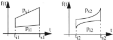
A high degree temporal band is, in general, mandatory to approximate an observation well. As we will see in section 3, our motivation to introduce polynomials of any degree in the temporal band definition is more to be able to process derivatives of higher order than to get a better approximation of an observation. That is the reason why we now define "temporal band sequences":

Definition 2: "Temporal band sequence"

A temporal band sequence SB is a finite ordered set of temporal bands {B1, .·. , Bnl such that:

where ti(B) is the initial instant of the band B and ts(B) the final instant.

The interval [ti(B 1), t 5 (Bn)[ is the temporal extent of the band sequence and the highest degree of the bands is the degree of the temporal band sequence.

We will denote by SB(t) = B(t) the value (an interval) of the temporal band sequence SB at the instant t (B is the temporal band of SB whose temporal extent contains t).

We can now define how to represent an observation:

Definition 3: "Representation of an observation "

A temporal band sequence SB whose temporal extent is [t1, t2[ is a representation of an observation v(t) over a time interval [t1, t 2 [ iff the observation is always encompassed within the bands, which means:

Example: the band sequences SB 1 and SB2 are two possible representation of v(t)

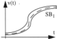
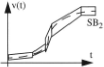
We have develop a procedure capable of computing a temporal band sequence given the information provided by the sensors (for example, a sampled signal). This procedure takes into account sensor inaccuracy in order to always properly represent the observation. It also makes a trade-off between the number of bands in the sequence, the inaccuracy introduced (characterized by the width of the band) and the degree of the bands. In case of observations made sequentially, it considers the temporal extent of the bands already computed in order to reduce the number of new bands possibly introduced by the "synchronization" operation defined below (Definition 5). So far, this procedure, based on the least squares method, generates band sequences whose degree is at most one; that does not make higher-degree bands irrelevant since such bands occur when combining first-degree bands together.

Definition 4: "Equivalence of temporal band sequences"

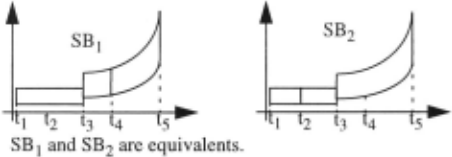
Two band sequences SB 1 and SB2 of same temporal extent [tl, tz[ are equivalent iff:

Hence, two equivalent temporal band sequences differ only in their temporal splitting.For example:

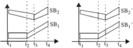
The synchronization of two temporal band sequences SB 1 and SB 2 whose temporal extents are the same consists in finding two temporal band sequences SB 1' and SB 2 ' such that:

• SB 1 and SB 1' (resp. SB2 and SB2 ') are equivalent,
• ISB1 'I= ISB2'1 = n

where SB[i] denote the i 1 h band of SB.

For example, SB' 1 and SB '2 have been made synchronous:

Property 1:

The minimal synchronization of two temporal band sequences whose temporal extents are the same always exists and is unique.

We now define the necessary operations to use the temporal band sequences formalism for components modeling.

Definition 6: "Sum of temporal band sequences"

The sum of two synchronous band sequences SB 1 and SB 2 of size n is the band sequence SB of size n such that:

where the sum of two bands (lj, ts, Pi I, Psi) and (ti, ts, Piz, Psz) is the band (lj, ts, Pil + Piz, Psi+ Pd

Property 2:

The sum of two band sequences maintains the property of representation; this means that, if any functions g 1 (t) and g2(t) are represented by temporal band sequences SB 1 and SB2 then the function g 1 (t) + g 2 (t) is represented by SB 1 + SB2.

Computing the sum of two temporal band sequences which are not synchronous consists in synchronizing these sequences and then computing their sum.

This definition is easily extended to the sum of a temporal band sequence and an interval.

·We now define the integral of a temporal band sequence. Our aim is to define a temporal band sequence representing the function r g(x)dx from the representation of the function g(t). e .

Definition 7: "Integral of a temporal band"

The integral of a temporal band B = (ti, ts, Pi , Ps) from any instant 8 belonging to the open interval (ti, ts) is a temporal band sequence {(ti, 8, Ps, Pj), (8, ts, Pi, Ps)}, noted I B, ru~ili~: e

We extend this definition for ti and ts such that

It can easily be proved that the constraint of the temporal band definition holds, that is:

We now recursively define the integral of a temporal band sequence.

Definition 8: "Integral of a temporal band sequence"

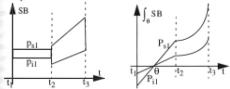
The integral from any instant 8 belonging to ]ti(B), ts(Bj)[ of a temporal band sequence SB = { B 1, ... , Bn} of size n and degree p is a temporal band sequence { B '1, .. . , B 'j-l} U {B'jl, BJ'jz} U {B'j+l , ... , B'nl of size n+l and degree p+l, noted SB, such that e

The constant B 'k+l (ts(Bk)) corresponds to the integration of the intermediate bands (Bj to Bk).

Thus, computing the integral of a band sequence SB consists in computing the integral of the /h band of SB, then computing the integrals of the j+ I th and j-1 th bands from the . I f h ·th mtegra o t e J , ...

Example:

Property 3:

The integration of a temporal band sequence maintains the property of representation; this means that, if any function g(t) is represented by a temporal band sequence SB then the function r g (x) dx is represented by f SB . (j (j

In the same way, we define the product of two temporal band sequences and the product of an interval and a temporal band sequence. In both cases, the property of representation is kept but the number of bands in the sequence and/or the degree of bands can increase. Complete definitions and proofs can be found in [Loiez 97] .

Any polynomial operation can be built from the previous definitions (sum and product) at the cost of an increase of inaccuracy when the same quantity occurs several times. Primitive operations can be defined to avoid this loss of accuracy as it is done with real functions in [Moore 66].

3 Diagnosing with Temporal Band Sequences

3.1 Principle

The diagnosis approach we propose takes place in the model based diagnosis theory [Reiter, 87]: each model is associated (by a conjunction of -,ab(.) predicates) with the set of components which allows one to assume the model of a component or a block of components holds. Diagnosing, then, consists in detecting the inconsistent models to determine the conflict sets (nogoods).

Definition 9: "Behaviour model of components"

We call correct behavior model of the components c1, c2, ... , cP' an expression of the form:

where f, g, h, k, ... are (any) temporal functions.

Allowing derivatives of any order in the model equation eases components modeling. In particular, the use of simulation models for diagnosing can be considered and also complex block modeling.

For example possible models are:

• a block composed of a capacitor c and an inductance 1:

Inverting definition 9 gives:

3t, f(t) + g'(t) + h" (t) + k'"(t) + ... :;t 0 :=:} ab(c 1 ) v .. . v ab(cn) Diagnosing then consists in determining for each model if:

Our main result is that there exists a procedure to make this computation in an efficient way when the temporal functions are represented by synchronous temporal band sequences. We shall now present this procedure.

3.2 An inconsistency detection procedure

Our idea is to represent each model expression f(t) + g'(t) + h" (t) + k"'(t) + ... by a temporal band sequence thanks to temporal band sequence operations defined in section 2. Directly representing the model expression would require an approximation at every instant, not only of observations but also of their derivatives, which is not easy to obtain for the first derivative (and is a limitation of the CATS system) and is unrealistic for higher order derivatives.

To overcome this problem, the model expression is transformed into an equivalent expression in order to be able to represent it by a temporal band sequence without having to approximate the derivatives at every instant. For that, we will take advantage of the fact that integrals of temporal band sequence are easy to compute. As the procedure depends on the degree of the equations, we present it for different cases:

Equations without any derivative:

Let a model equation f(t) = 0 and SB a temporal band sequence representing f(t). As the value of the function f(t) is known (0), it is possible to verify if f(t) is really represented by SB. If it is not the case, the model is inconsistent. Thus, directly using equation (2) gives:

The procedure consists in verifying if this relation holds.

Model equations without any derivative are not a rare occurrence. For example, checking the inconsistency of the equation vr = R ir of a resistor model whose quantities vr and ir are respectively represented by the temporal band sequences SBV and SBI consists in computing the temporal band sequence SBV - R SBI and checking if the relation (3) holds.

First Order Equation:

Let a model equation f(t) + g'(t) = 0 and SBf, SBg the temporal band sequences representing respectively f(t) and g(t). It is not possible to compute a temporal band sequence representing g'(t) from SBg. For that reason, we integrate the model equation. This gives :

• choosing an integration instant 8 (this choice will be dis­ cussed in section 4.1 ),

• computing the temporal band sequence JsBf+SBg-SBg(9) which represents the function: 8

• checking the consistency of the equation without any deriv­ ative k(t) = 0.

Hence, checking the consistency of a first order equation consists in integrating once the equation and then checking the consistency of an equation without any derivatives.

Moreover, the fact that all the operations maintain the property of representation allows us to ensure that no false conflict will be detected.

Second Order Equation:

Let a model equation f(t) + g'(t) + h"(t) = 0 and SBf, SBg, SBh the temporal band sequences representing respectively f(t), g(t) and h(t). For the same reason as before, we integrate the equation from an instant e:

\it, f(t) + g'(t) + h" = 0

Thus, ~he procedure consists in:

• choosing an integration instant e,
• approximating the constant h'(8) by an interval H,
• computing the temporal band sequence J SBf + SBg- SBg(8)- H which represents the function ket) = f f(x)dx + g(t)- g(e) - h'(8), .
• checking 8 the consistency of the first order equatiOn k(t) + h'(t) = 0.

Hence, checking the consistency of a second order equation consists in integrating once the equation and then checking the consistency of a first order equation.

For the same reason as before, no false conflict set will be detected. However, the consistency of a second order equation f(t) + g'(t) + h "(t) = 0 can be checked only if an approximation of h' at time e can be obtained; this point is discussed in section 4.

Generalization:

In the same manner, equations of any order can be checked.

The procedure to check the consistency of a nth_order equation consists in:

• choosing an integration instant e,
• integrating once the equation,
• approximating the values of the derivatives which appear,
• computing the temporal band sequence which represents the function involving no derivatives,
• checking the consistency of the resulting n-1 th -order equa­ tion.

4 Discussion

The use of the consistency checking procedure just described for diagnosing analog systems raises two main questions related to the integration instant e and the compositionality of the approach. We discuss these two points here.

4.1 Integration instant

For first-order equations any integration instant can be chosen; nonetheless, inconsistency of the equation k(t) = 0 can be missed since the integration process adds inaccuracies and the (possibly) only instant when this inconsistency can be found out might be far from the chosen e . Hopefully, when only temporal bands of degree 1 are considered, an analytic procedure can be devised for checking equation k(t) = 0, as shown in [Loiez and Taillibert, 96a]. This procedure computes whether there exists at least one e for which the equation is inconsistent; it can be extended for bands of higher degree at the cost of some efficiency since it then requires solving numerically polynomial equations.

Another difficulty occurs for equations with second order derivatives: an approximation of the first derivative of function h(t) at time e is mandatory. This approximation can not be computed from the temporal band sequence representing h(t), but must be obtained from observations (as is the case in CATS). We have said that it is difficult to approximate a function derivative at every instant, but the fact that we just have to approximate it at only one instant (9) makes that problem less critical. For example, it is often possible to choose an instant for which the system is stable, i.e. an instant when all derivatives are zero. The same reasoning applies for equations with higher order derivatives. Hence, for these equations, the choice of the integration instant e is imposed by the need to have an approximation of derivatives at that time. That may be a cause of incompletness since this constraint can conflict with the one mentionned just above. Experiments carried out so far do not suggest that this problem could be a serious impediment for a practical use of our method.

4.2 Compositionality

Thanks to the temporal band sequences formalism just described, we can represent observation of quantities which continuously evolve in time. The modeling we have suggested allows the description of components by equations like f(t) + g'(t) + h" (t) + .. . = 0 where f, g, h, ... are functions involving quantities of the system to be diagnosed and sum and product operations .

However, the procedure we have presented can only detect inconsistencies - and hence find out conflicts - if a temporal band representation of all the functions of an equation is available. But, in general, not all the physical quantities of the system to diagnose are measurable. (For example, currents in electronics). If these quantities are involved in the functions of the equation, the consistency of the corresponding model will not be checked.

Moreover, the consistency checker tests the models one by one and independently of one another; to detect all the possible conflict sets with as few measurements as possible we need some composition of models.

To solve these problems, a classical propagation procedure is applicable: when temporal band sequences for a quantity and its derivative are predicted -say v and v' -, consistency is checked with the procedure described in section 3-2 for f+g'=O (by making f=v' and g=-v).

In DOGS, the program we developed to experiment Temporal Band Sequences, we tried another approach by generating off-line all possible equations of the form f(t) + g'(t) + h "(t) + ... = 0 and such that the quantities present in the functions f, g, h, ... are measurable; all possible combination of these equations eliminating some quantity are also computed 1 .

We notice that the theoretical complexity of such an algorithm is huge (more than 2" generated equations where n is the number of components). But, in practice, the number of equations remains manageable when circuits are weakly connected (few equations contain the same quantity) or when the number of measurable quantities is low compared to the total number of quantities (about 50% in electronics). Moreover, if we impose a limit to the size of the conflicts to be detected, the number of the resulting equations should remain "reasonable".

5 Conclusion

The approach that we have presented has been essentially motivated by our need to represent observations such as signals which vary continuously over time and to use them for diagnosis purpose.

In [Loiez and Taillibert, 96a], Temporal Band sequences were limited to first order temporal bands (trapezoid) which was already a real improvement w.r.t. the result obtained with the CATS system, especially when fast varying signals were considered. The extension to polynomial temporal bands seems quite natural but we have had the pleasure to find out that it allowed not only a better approximation of signals, but mainly, that it also allowed one to take into account derivatives of higher order and more complex operations, and hence, ease the component modeling. The only constraint is to get an approximation of derivatives at one instant for which approximation is safe.

The temporal band sequence operations process can increase the number of "episodes" but, this drawback is limited since we do not propagate these new episodes.

Various extensions to the procedure generating the models can be imagined; for instance, we associate preconditions to models in order to allow a piecewise linear description and hence to ease modeling of complex components such as diodes or transistors 2 .

DOGS has been tested with first degree bands, on the monostable circuit chosen as a reference problem by the diagnostic community [Dague and Taillibert, 96]. The results obtained by CATS on the same circuit [Dague et al, 90] are the same with DOGS without the risk of faulty diagnosis due to the computation of derivatives made by CATS in the fast­ varying part of signals. Moreover, DOGS has given good results with second order circuits like filters.

I. DOGS processes only linear functions; it eliminates unmeasura­ ble quantities by a gaussian elimination and generates all the equa­ tions by considering all the possible pivotal elements

2. As in CATS, equations modeling such components are given by experts and rely upon high-level parameters (gain, ... ).

Acknowledgments

E.Loiez work is supported by the "Conseil General du Nord­ Pas de Calais". A preliminary version of that work was presented in [Loiez and Taillibert, 96b].