
Generalized Physical Networks for Automated Model Building
Proceedings of the Sixteenth International Joint Conference on Artificial Intelligence. Qualitative Reasoning and Diagnosis. Pages 1047-1052.
© 1999 International Joint Conferences on Artificial Intelligence
Abstract
We pr ese nt a new knowledge representation and reasoning framework for mod eling nonlinear dynamical systems. The goa ls of this framework are to smoothly incorporate varying levels of domain knowledge and to tailor the reasoning methods - and hence th e search space - accordingly. Our solution exploits generalized physical networks (GPN), a meta-level representation of idealized two-terminal elements, tog et her with a hierarchy of qualitative and quantitative analysis tools, to produce a dynamic modeling domain whose complexity naturally adapts to the amount of available information about the target system.
- [Addanki et al., 1991] S. Addanki, R. Cremonini, and J. S. Penberthy. Graphs of models. Artif. Intel., 51:145-178, 1991.
- J. Amsterdam. Automated Qualita- tive Modeling of Dynamic Physical Systems. MIT AI Lab, Cambridge, MA, 1992. Tech. Report 1412.
- [Bobrow et al., 1996] B. Bobrow, B. Falkenhainer, A. Farquhar, R. Fikes, K. Forbus, T . Gruber, Y. Iwasaki, and B. Kuipers. A compositional modeling language. In QR-g6, 1996.
- [Bradley and Stolle, 1996] E. Bradley and R. Stolle. Au- tomatic construction of accurate models of physical systems. Annals of Math. & Artif. Intel., 17:1-28, 1996.
- [Bradley et al., 1998] E. Bradley, A. O'Gallagher, and J. Rogers. Global solutions for nonlinear systems using 1052 QUALITATIVE REASONING AND DIAGNOSIS qualitative reasoning. Annals of Math. & Artif. Intel., 23:211-228, 1998.
- [Capelo et al., 1998] A. C. Capelo, L. Ironi, and S. Ten- toni. Automated mathematical modeling from experi- mental data: an application to material science. IEEE Transactions on Systems, Man and Cybernetics -Part c, 28(3):356-370, 1998.
- [Casdagli, 1992] M. Casdagli. A dynamical systems ap- proach to modeling input-output systems. In Nonlin- ear Modeling and Forecasting. Addison-Wesley, 1992.
- [Falkenhainer and Forbus, 1991] B. Falkenhainer and K. Forbus. Compositional modeling. Artif. Intel., 51:95-143, 1991.
- [Hsu, 1987] C. S. Hsu. Cell-to-Cell Mapping. Springer, New York , 1987.
- [Karnopp et al., 1990] D. Karnopp, D. Margolis, and R. Rosenberg. System Dynamics: A Unified Ap- proach. Wiley, New York, 1990. 2nd edition.
- [Kuipers, 1986] B. Kuipers. Qualitative simulation. Ar- tif. Intel. , 29(3):289-338, 1986.
- [Mauss and Neumann, 1996] J. Mauss and B. Neu- mann. Qualitative reasoning about electrical circuits using serial-parallel-star trees. In QR-g6, 1996.
- [Masterman and Biswas, 1997] P. Masterman and G. Biswas. Formal specifications for hybrid dynamical systems. In IJCAI-g7, 1997. IJCAI
- [Paynter, 1961] H. M. Paynter. Analysis and Design of Engineering Systems. MIT Press, Cambridge, MA, 1961.
- [Sanford, 1965] R. Sanford. Physical Networks. Prentice-Hall, 1965.
- [Sauer et al., 1991] T. Sauer, J. A. Yorke, and M. Cas- dagli. Embedology. J. of Statistical Physics, 65:579- 616, 1991.
- [Stolle and Bradley, 1998] R. Stolle and E. Bradley. Multimodal reasoning for automatic model construc- tion. In AAAI-gs, 1998.
- [Strogatz, 1994] S. Strogatz. Nonlinear Dynamics and Chaos. Addison-Wesley, 1994.
- [Top and Akkermans, 1991] J. Top and H. Akkermans. Computational and physical causality. In IJCAI-gl, 1991. IJCAI
- [Weld and de Kleer, 1990] D. Weld and J. de Kleer, ed- itors. Readings in Qualitative Reasoning About Physi- cal Systems.
- Morgan Kaufmann, San Mateo CA, 1990.
- [Weld, 1992] D. Weld. Reasoning about model accuracy. Artif. Intel., 56:255-300, 1992.
- [Williams and Nayak, 1996] B. Williams and P. Nayak. A model-based approach to reactive self-configuring system. In AAAI-g6, 1996.
References were extracted automatically from the PDF and may contain errors.
Full text extracted automatically from the PDF; figures, tables and equations may differ. The PDF is the version of record.
1 Introduction
System identification (SID) is the process of identifying a dynamic model of an unknown system. The topic of this paper is a new knowledge representation and reasoning (KRR) fra!llework that makes it possible to automate this kind of analysis. The challenges involved are sig nificant. Applications in different fields of science and engineering demand different kinds of models and mod eling techniques. Large aerospace structures, for exam ple, usually have a variety of inputs (wind speed, engine thrust, and turbulence) and outputs (velocity, stress and strain indicators from wing sensors, etc.) and are de scribed by partial differential equations; a simple electri cal circuit, on the other hand, may have a single current source as an input and a voltmeter as an output, and can be described by an ordinary differential equation (ODE) . Any representation designed for reasoning about models of such systems has to be both flexible enough to han dle various degrees of uncertainty and complexity, and yet powerful enough to deal with situations in which the input signal may or may not be controllable.
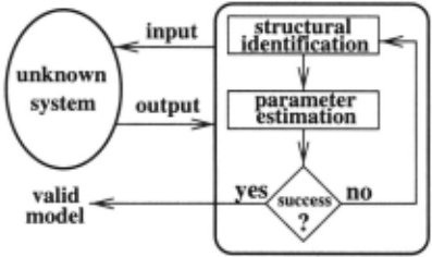
System identification entails two steps, as shown in Fig. 1: structural identification, wherein one ascertains the general form of the model (e.g. , the ODE a1B + a2 sinO = 0 for a simple pendulum), and then parameter estimation, in which one finds specific pa rameter values for the unknown coefficients that fit that model to the observed data (e.g. a1 = 1.0, a2 = -98.0) . Both steps depend upon input-output analysis[Casdagli, 1992], wherein the relationship between drive and re sponse is used to infer useful information about inter nal system dynamics. For nonlinear systems, param eter estimation is difficult and structural identification is even harder; AI techniques can be used to automate the former[Bradley et al. , 1998], but the latter has, until now, remained the purview of human experts.
*Supported by NSF NYI #CCR-9357740, ONR #N0001496-1-0720, and a Packard Fellowship in Science and Engineer ing from the David and Lucile Packard Foundation.
A central problem in any automated modeling task is that model complexity- and hence the size of the search space - is exponential in the number of model frag ments unless severe restrictions are placed on the model building process. Ideally, one would like to build black box models using general reasoning techniques that ap plied to any system and did not require any domain knowledge about the system under examination. The combinatorics of the generate phase make this an unre alistic paradigm. A useful alternative is gray-box model ing, where the "box" is not completely opaque and infor mation about its internals can used to prune the search space down to a reasonable size. Some automated model ing tools, for example, maintain a library of typical com ponents for a particular domain and build models by try ing out various combinations of those primitives[Capelo et al., 1998]. This approach is useful in relatively simple domains where the relationship between idealized mod eling components and actual physical components is well known. Most AI modeling work has taken a clear-box modeling approach, in which one knows almost every thing about what one is trying to model. The goal of the work described in this paper is to develop a KRR framework that supports automated modeling in a range of gray shades that is useful to practicing engineers.
The key to making gray-box modeling of nonlinear dy namical systems practical is a flexible knowledge repre sentation scheme that adapts to the domain generality. Domain-dependent knowledge can reduce search-space size, but its applicability is fundamentally limited; the challenge in balancing these influences is to be able to determine, at every point in the reasoning procedure, what knowledge is (1) applicable and (2) useful. Knowl edge that a particular input voltage controls an output frequency, for instance, allows one to reason more ef fectively about manipulating that voltage to learn more about the system.
The solution proposed here combines a representation that allows for different levels of domain knowledge, a set of reasoning techniques appropriate to each level, and a control strategy that invokes the right technique at the right time. In particular, we combine ideas from gen eralized physical networks[Sanford, 1965], a meta-level representation of idealized two-terminal elements, with traditional compositional model building[Falkenhainer and Forbus, 1991] and qualitative reasoning[Weld and de Kleer, 1990]. The intent is to bridge the gap between highly specific KRR frameworks that work well in a sin gle, limited domain (e.g., a spring/ dash pot vocabulary for modeling simple mechanical systems) and abstract frameworks that rely heavily upon general mathemat ical formalisms at the expense of having huge search spaces[Bradley and Stolle, 1996]. The generalized phys ical network (GPN) representation is an effective way to construct a description that is appropriate to a wide range of points on this spectrum, and thus it provides a useful bridge between general and specific modeling approaches.
2 Generalized Physical Networks
In the late 1950s and early 1960s, inspired by the real ization that the principles underlying Newton's third law and Kirchhoff's current law were identicaP, researchers began combining multi-port methods from a number of engineering fields into a generalized engineering domain with prototypical components[Paynter, 1961]. The basis of this generalized physical networks (GPN) paradigm is that the behavior of an ideal two-terminal element - the "component" - may be described by a mathematical re lationship between two dependent variables: generalized flow and generalized effort, where fiow(t) * effort(t) =
1 Summation of {forces, currents} at a point is zero, re spectively; both are manifestations of the conservation of energy.
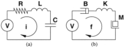
power(t). This pair of variables manifests differently in each domain: (flow, effort) is (current, voltage) in an electrical domain and (force, velocity) in a mechanical domain 2 . One of the strengths of the GPN representa tion is that it brings out similarities between components and properties in different domains. Electrical resistors ( v = iR) and mechanical dampers ( v = J B) are analo gous, as both dissipate energy. Similar relationships ex ist for generalized inertia, capacitance, flow, and effort source components, as shown in Table 1; see [Karnopp et al., 1990] or [Sanford, 1965] for mechanical rotational, hydraulic, and thermal domains. Relationships also ex ist for pairs of mutually coupled two-terminal elements, such as electrical transformers or differential gears, in which a flow or effort in one element induces a flow or effort in the other. Components may be connected in the standard network-theoretic ways - parallel, serial, star, delta, etc. - and the network topology need not be planar.
| Component | Electrical | Mechanical Translation |
| Resistor | v = Ri | v=Bf |
| Capacitor | i = c~~ | f=M~~ |
| Inertia | v - ·uti. - dt | v=Ktt |
| NL Resistor | v = -RAi., | v= -RAJ"' |
Utilizing a small number of these primitive elements, GPNs can effectively model systems in a wide variety of domains; moreover, they make it very easy to in corporate varying amounts of information about those domains. A GPN-based modeling domain consists of a set of components and a set of connection primitives ("connectors"); a G PN model is a specific instance of connected components- e.g., a series connection of an inertia, a resistor, and a capacitor- represented by an incidence matrix. The same GPN model can be ab stract and general or highly specific, depending on how much one knows about the domain. Both of the net works in Fig. 2, for example, can be modeled by a se ries inertia/resistor/capacitor GPN; knowledge that the system is electronic or mechanical would let one refine the model accordingly. The available domain knowledge, then, can be viewed as a lens that expands upon the in ternals of some GPN components, selectively sharpening the model in appropriate and useful ways.
There are a variety of ways to use generalized physical networks to help automate the structural identification phase of the SID process. One could, for example, create a library of all known components, enumerate all pos sible component combinations/configurations, and test each member of this succession until a valid model is found. This method is obviously impractical, as sim ple enumeration creates an exponential search space - a severe problem if the component library is large, as must be the case if one is attempting to model nonlinear systems 3 . A more-intelligent idea is to use a hierarchy of domain-dependent and -independent knowledge to direct the search, as described in the following section.
2 In bond graphs[Karnopp et al., 1990], another general ized representation paradigm, velocity is a flow variable and force is an effort variable. The difference between GPNs and bond graphs is only a frame-of-reference shift.
3 Reasoning with GPNs
The GPN representation, as described in the previous section, is an effective basis for a dynamic modeling do main whose complexity naturally rises and falls accord ing to the available information about the target sys tem. A general domain - e.g., {all dynamical systems} - has a complex search space; a specific domain like {conservative mechanical systems} has a much smaller one. The challenge in reasoning about GPN models is to tailor the reasoning to the knowledge level in such a way as to prune the search space to the minimum. Or ganizing domains into a hierarchy of generality - e.g., {dynamical systems, electromechanical systems, mechan ical systems, conservative mechanical systems, ... } - is not enough; what is needed is a hierarchical set of anal ysis tools, as well as a means for assessing the situation and choosing the appropriate tool.
Naively speaking, the goal is to start with a "plausi ble" model and then move through the space in a "rea sonable" fashion. The key to doing so is to classify model and system behavior at an appropriate qualitative level. The order of an ODE, for instance, contains some use ful high-level information about its behavior, and that kind of simple symbolic information can be used to re move huge branches from the search space. Sometimes, however, pruning a single leaf off the search tree re quires expensive operations like point-by-point compar isons of ODE solutions to sensor data sets. Orchestrating this process efficiently is a difficult problem; its solution requires powerful machinery like theorem-provers and declarative meta-level control[Stolle and Bradley, 1998]. The generality of any behavior classification tool is also affected by the domain of the target system; phase portrait and time-series analysis apply to all ODEs, for instance, but transient analysis designed to detect "ir recoverable viscous deformation" is only meaningful for viscoelastic systems.
3 Nonlinear terms are somewhat idiosyncratic, and each must be supplied as a separate library entry. This issue has not arisen in previous work on GPNs because their use has been generally confined to linear systems.
The KRR framework described in this paper is de signed to exploit domain knowledge in order to navigate effectively through the search space of ODE models. The basic idea is that different reasoning techniques are ap propriate to different domains, and the key to the solu tion is that the GPN component type and domain knowl edge dictate which one to use. Table 2 shows part of the hierarchy of analysis tools that we have implemented. The top category is the broadest and most general. Lin-
| I System Type | Analysis Tools |
|---|---|
| Nonlinear | Cell-to-cell-mapping Delay-coordinate embedding NL time series analysis |
| Linear | Linear system analysis |
| Restricted linear | Domain dependent |
ear systems are a subset of nonlinear systems; restricted linear systems - which use distributed parameters to model systems in very specific physical domains 4 - are, in turn, subsets of linear systems. Analysis tools that apply to any of these groups obviously apply to its sub sets as well. All of the nonlinear systems tools listed in Table 2 work with the phase-space representation. Cell-to-cell mapping[Hsu, 1987] is a geometric reasoning technique that classifies a phase portrait qualitatively using simple discretized heuristics. Delay-coordinate embedding[Sauer et al., 1991]lets one infer the dimen sion and topology of the internal system dynamics from a time series measured by a single output sensor. Non linear time-series analysis is a blanket term for classi fication that follows the { attractors, bifurcations, ... } ontology of nonlinear dynamics[Strogatz, 1994]. Linear systems analysis refers to the techniques taught to undergraduate engineers (step/frequency response, etc.) . Analysis tools for restricted linear systems - e.g., creep testing - are highly domain-specific.
Reasoning about models proceeds in the obvious man ner, given this hierarchy: if no domain knowledge about the target system is available (i.e., the true "black-box" situation), then models are constructed, analyzed, and compared to the target system using general reasoning techniques that apply to all ODEs. Constructing models in this highly general manner is difficult, as there is no domain knowledge to limit the search, but it is also universally applicable. If the system is known to be linear, the extensive and powerful repertoire of linear analysis tools developed over the last several decades makes the task far less imposing. Among other things, system in puts (drive terms) in linear systems appear verbatim in the resulting system ODE, which makes input/output analysis much easier. In restricted linear domains, anal ysis tools are even more specific and powerful. In vis coelastics, for example, three qualitative properties of a "strain test" reduce the search space of possible models to linear.
4 e.g. modeling electrical transmission-line loss through se ries connections of multiple RC circuits; see Section 5 for an example in the viscoelastic domain.
Given all of this machinery, we build models as fol lows. First, a candidate GPN model is constructed us ing a basic subset of the components and connectors of a particular domain. This process is guided by the anal ysis tools in Table 2. The cohort of nonlinear tools, for example, is first applied to the sensor data to determine the dimension d of the dynamics; this fact allows the modeling tool to automatically disregard all models of order < d. We have currently implemented roughly a dozen other nonlinear analysis techniques that yield sim ilar search-space reductions; if the system is linear, sev eral dozen more tools apply as well. Knowledge that the target system is oscillating, for example, not only con strains the model to be of least second order, but also im plies some constraints on its coefficients. If this reduced search space does not contain a model that matches the observed system behavior, the GPN modeling domain is dynamically expanded to include more esoteric compo nents. For example, if all models in the {linear-inductor, linear-resistor} domain are rejected, then the domain might be expanded to include linear-capacitors. Once a successful GPN network is found, the final step in the model-building process is to convert it into ODE format, as described in the following section.
4 Converting GPNs to ODEs
The last stage in the system identification process is to convert the domain-independent GPN model into ODE form. This conversion step is fairly easy to automate. The powerful network-theoretic principles involved have been in the engineering vernacular for many decades, but we use them in a very different manner. Tradition ally, one applies a tool like modified nodal analysis> to a known network with known component values in or der to analyze or simulate its behavior. We use loop and node equations to convert a GPN network with un specified component values into an ODE (also with un specified component values). Finally, we use a nonlinear parameter estimator[Bradley et al., 1998] to find compo nent values that match that ODE model to the observed system behavior. In this section, we describe how this procedure works for the electronics domain; the process is effectively identical in other domains.
The GPN---+ODE algorithm is similar to standard sys tem analysis: create a set of loop or node equations, sub stitute physical component models into those equations, and then simplify /change variables as necessary. This al gorithm is significantly simpler than a comparable bond graph---+ODE conversion algorithm, since a bond graph algorithm creates implicit causal orderings as it creates the set of ODEs.
5 which is based on node equations
Algorithm:
- Use generalized Kirchhoff's current law - L,{fiows into a node} = 0 - to identify l independent branch currents, l = b- (n- 1) , where b is the number of branches and n is the number of nodes in the net work. Branch independence is guaranteed by choos ing each successive loop such that it traverses one and only one branch that is not part of an existing loop. The branches of a depth-first search tree of the network form one such set.
- Use generalized Kirchhoff's voltage law-'£,{ efforts around a loop} = 0 - around each of the l closed loops identified in step 1, yielding l system equa tions.
- Apply the correct effort/flow relationships (from Ta ble 1) to every element in the l loops from step 2, creating a set of ODEs.
- Use variable substitution and/or symbolic differen tiation to remove integrating elements as necessary.
As an example, consider a GPN modeling domain that allows parallel and serial connections of linear resistors (R), inductors (L), and nonlinear active resistors (NR) that obey the constitutive relation v = -RAi 3 + Rsi . Midway through the procedure, after the modeler has tried and rejected a variety of too-simple models, we might see the candidate model shown in Fig. 3. Since
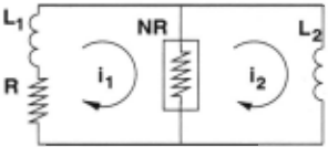
b = 4 and n = 3, two loops are required. These are chosen automatically from the branches of a depth-first spanning tree. i1 and i2, as shown, are one possibility; i1 and a loop through {R, L1 , L2 } are another. Using gen eralized KVL around these two loops and substituting the given component models yields:
The last step is to pass this set of independent system equations in the two state variables { i 1, i2} to the pa rameter estimator for comparison with observed behav ior and determination of the unknown coefficients £ 1 , R, etc. If the model fails this check, the modeling tool first tries to reconfigure it (e.g. moving L1 to be in series with NR instead of R), and eventually gives up and expands the modeling domain (e.g. including linear ca pacitors). This generate-and-test process continues until a valid model is found.
This technique may initially appear to be a simul ation/ diagnostic tool for a system whose structure is completely known, but it is really much more abstract and adaptable. The KRR framework lets the modeling tool work with general GPN components as long as pos sible: up until the point when it converts the network into a set of ODEs. The relationships between compo nent models and actual components of a physical system are a wholly separate data structure.
This approach has several important limitations and restrictions. Among other things, these models do not explicitly represent causality relationships - informa tion that is very important for diagnostic tasks or au tomated explanation tools, but less so for system iden tification. The algorithm described above can also cre ate extra system equations and variables; it may, for in stance, construct a large resistive network when a single Thevenin equivalent would do. One can solve this prob lem using resistive network reduction[Mauss and Neu mann, 1996]; we avoid it from the outset by building models in a sequential fashion and not adding like com ponents in serial or parallel. Other meta-level represen tational schemes (such as bond graphs) solve these prob lems automatically, but GPNs are more expressive and more widely applicable, as well as easier to implement and use.
As is true of automated modeling in general, evaluat ing the results of this approach can be difficult because the question "How is this model better?" is hard to formalize. From an engineering standpoint, a successful model is one that matches observed behavior to within predefined specifications. PRET, the automated model ing tool in which these ideas are instantiated, is designed to be an engineer's tool, so its judgement of what con stitutes success or failure is exactly that. Parsimony is another desireable attribute in a model: one wishes to account for the observed behavior using as few - and as simple- ODEs terms as possible. Defining good met rics for model fragment simplicity is deceptively difficult, and it remains an open problem in automated modeling community. Finally, the speed with which PRET pro duces such a model is another important metric, partic ularly as we work with more-complex systems and search spaces. Ultimately, the best form of evaluation will con sist of whether or not PRET's models are useful for con trol system design - that is, whether the ODE that PRET constructs of a radio-controlled car can actually be used as the heart of a controller designed to direct that car to perform some prescribed action. We are in the process of evaluating models of real-world systems in several domains - ranging from robotics to hydrology
- in this manner.
5 Related Work
Much of the pioneering work in the qualitative reasoning (QR) modeling community focuses on reasoning about pre-existing models: simulating them[Kuipers, 1986], simplifying and refining them[Weld, 1992], or keeping track of which model is appropriate in which regime[Ad danki et al., 1991]. QR model construction research has focused on building models from fragments[Falkenhainer and Forbus, 1991; Bobrow et al., 1996; Williams and Nayak, 1996; Capelo et al., 1998]. The work described in this paper uses some of the same techniques, but it has different goals and a different overall approach: it works with noisy, incomplete sensor data from real-world systems and attempts not to "discover" the underlying physics, but rather to find the simplest ODE that can account for the given observations.
Of all the QR modeling work cited in the previous paragraph, [Capelo et al., 1998] is the most closely re lated to this paper. Capelo et al. build ODE models of linear viscoelastic systems by evaluating time series using qualitative reasoning techniques, and then use a parameter estimator to match the resulting model with a given system. This domain is limited - a "restricted linear system," in our terminology - and fairly simple; it involves only two component types (linear springs and dashpots), connected in series and/or parallel. The spe cific nature of the domain naturally limits the search space, so a simple qualitative pre-processing step can be used to identify the system as one of only four differ ent model types. The system described in this paper is much more general; it works on all linear and nonlinear lumped-parameter continuous-time ODEs and uses dy namic model generation to handle arbitrary devices and connection topologies in multiple domains. (Indeed, one of the domains that we have implemented is {viscoelastic systems}.)
The representation most closely related to GPNs is the bond graph[Karnopp et al., 1990]. In the QR lit erature, bond graphs have been used primarily for rea soning about causality[Top and Akkermans, 1991] and modeling hybrid systems[Mosterman and Biswas, 1997]. An important exception to this is Amsterdam's work on automated model construction in multiple physical domains[Amsterdam, 1992], which uses bond graphs to model linear systems of order two or less. While bond graphs are a good alternative to generalized physical networks - especially if causality issues are a concern -converting them into ODE models is difficult, which makes them less useful for the kinds of complex nonlinear modeling tasks that we address in this paper.
6 Conclusions and Future Work
Generalized physical networks, coupled with a hierarchy of qualitative and quantitative reasoning tools that re late observed physical behavior and model form, provide the flexibility required for gray-box modeling of nonlin ear dynamical systems. This type of reasoning, wherein the modeling tool has only partial knowledge of the internals of the target system, accurately reflects the ab straction levels and reasoning processes used effectively by human engineers during the modeling procedure. The KRR framework described in this paper allows auto mated modeling tools to reason effectively with varying levels of domain knowledge - about different domains and at different levels of abstraction in an individual domain. The GPN component representation adapts naturally to the information available about the target system, allowing for the creation of dynamic modeling domains. Detailed knowledge automatically reduces the search space of models and triggers powerful, specialized reasoning techniques that are appropriate for that situ ation; in the absence of such knowledge, the system falls back on broadly applicable domain-independent princi ples to navigate through an exponential search space.
Besides speeding model generation, this KRR frame work streamlines reasoning about the relationship be tween input sources and output responses. We are cur rently working on automating this kind of reasoning, us ing GPNs to represent sensors and actuators explicitly with the goal of automatically performing experiments on unknown systems. vVe are also investigating model fragments and model complexity. Our domain libraries currently include linear components and some simple nonlinear ones; if the modeling task calls for a more complicated device, we first query the user and then re sort to power-series expansions. Once we have experi mented with more nonlinear systems in more domains, we may augment our libraries, and it may be useful to organize them in hierarchies (e.g. one linear spring as a starting point, with a simple nonlinear spring as an alternative, and more-complicated devices further down the hierarchy).
Acknowledgments: Reinhard Stolle, Joe Iwanski , Apollo Hogan, and Brian LaMacchia also contributed code and/or ideas to this project, and the IJCAI review ers' comments helped focus the content of this paper.
@inproceedings{ijcai1999p149,
  title     = {Generalized Physical Networks for Automated Model Building},
  author    = {Easley, Matthew and Bradley, Elizabeth},
  booktitle = {Proceedings of the Sixteenth International Joint Conference on
               Artificial Intelligence, {IJCAI-99}},
  publisher = {International Joint Conferences on Artificial Intelligence},
  editor    = {Thomas Dean},
  pages     = {1047--1052},
  year      = {1999},
  note      = {Qualitative Reasoning and Diagnosis},
  url       = {https://ijcai.org/proceedings/1999/149},
}
TY - CPAPER TI - Generalized Physical Networks for Automated Model Building AU - Easley, Matthew AU - Bradley, Elizabeth T2 - Proceedings of the Sixteenth International Joint Conference on Artificial Intelligence, IJCAI-99 PB - International Joint Conferences on Artificial Intelligence PY - 1999 SP - 1047 EP - 1052 UR - https://ijcai.org/proceedings/1999/149 ER -Copied
Machine-readable versions of this paper, for tools and AI agents:





