Formal Specifications for Hybrid Dynamical Systems

1 Introduction

Physical systems are inherently continuous and their be­ haviors are governed by the principles of conservation of energy and continuity of power [3] . Perceived disconti­ nuities are in reality fast nonlinear continuous behaviors. For efficient analysis, the differences in time scale may be exploited so that the nonlinear behaviors can be ab­ stracted to manifest as ideal discontinuities at points in time. An example is an ideal elastic collision between a body and a floor where the velocity of the body re­ verses instantaneously on impact . In reality, the colli­ sion occurs on a small time interval during which kinetic energy is converted into potential elastic energy, which then reverts back completely to kinetic energy for the body. Discontinuous effects can also be created by pa­ rameter abstraction [5] . Small parasitic physical effects that cause nonlinear continuous effects are abstracted away to simplify system description. For example, an ideal non-elastic collision between two bodies involves instantaneous discontinuous changes in velocity for the two bodies at the point of impact. A more precise model would have included small elasticity coefficients for the two bodies, and the period of impact would be a small but finite time interval , in which the change in veloci­ ties for the bodies would occur in a continuous manner. Models that combine continuous and discrete effects are called hybrid systems.

During discontinuous changes, physical laws of conser­ vation of energy and continuity of power may be violated [5]. In such situations, the initial state vector following the discontinuous changes is computed using the princi­ ple of conservation of state along with explicitly modeled interactions with the environment. In previous work [5; 7], this theory of discontinuous configuration changes in physical system models has been developed into a hybrid bond graph modeling paradigm that combines traditional bond graph elements with ideal switching elements con­ trolled by finite state automata. Formal schemes for ver­ ifying the correctness of models based on the principle of divergence of time have also been developed [7] . The hybrid bond graph formalism can be effectively applied to systematically design and analyze hybrid models of dynamic physical systems. This paper focuses on de­ veloping a formal semantics for analyzing systems with mixed continuous/discrete components.

2 A Hybrid Modeling Paradigm

Hybrid models operate in continuous modes (typical physical system behavior), but at points in time when signal values cross pre-defined thresholds or when ex­ plicit external (control) events are imposed on the sys­ tem, changes in model configurations cause discrete changes in system behavior. An important observation is that the temporal trajectory of system behavior be­ comes piecewise continuous, where simple discontinuities can occur only at well-defined points in time. The key to developing a correct modeling paradigm is to ensure that interaction between the continuous and discrete model­ ing formalisms is unambiguous, rigorous, and consistent.

2.1 General Hybrid Dynamic System

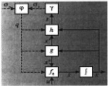
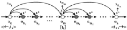
The general architecture for a hybrid dynamic system model (Fig. 1) can be specified by the 9-tuple:

H =< I, E, ¢,X, U,/a, g, h, 'Y > . Each mode of con­ tinuous behavior is given a unique state label O:k E I. Continuous behavior is governed by field !ak which de­ termines the continuous state vector Xak. The function h computes signal ( s E S) values from the state vector Xak in mode O:k, which may generate discrete events E specified by a mapping 'Y. 'Y is usually defined in terms of signal values reaching or crossing pre-specified thresh­ old values. Occurrence of a discrete event suspends the continuous behavior mode ak, and a new mode, ak+l, is generated by the discrete transformation ¢. The func­ tion g computes a new state vector, x+, for the new operational mode ak+l using values of the continuous state vector Xak in the previous operational mode ak.

2.2 The Continuous Model

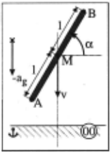
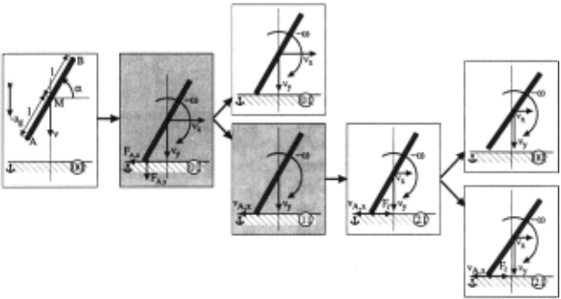
Dynamic physical system models are best represented as a set of differential equations on the system state vector. For example, the falling rod in Fig. 2 can be described by three state variables, the rod's linear velocities, v., and vy, and its angular velocity, w. When it is falling freely, only gravity acts on the center of mass and accelerates vertical movement. This can be described by the differ­ ential equation w = 0, v., = 0, Vy = ag, where ag is the gravitational acceleration.

Differential equation state space models, supple­ mented by algebraic constraints (DAEs) directly reflect underlying physical principles such as Kirchhoff's laws and phenomenological relations like Ohm's law. Many model parameters have an immediate physical meaning and equations can be systematically derived from bond graphs, network representations, and block diagrams [2] . A general representation of an ODE model derived from DAEs is: x(t) = !a(x(t), u(t), t) . The field, Ia, describes continuous temporal evolution of system behavior in a mode of operation, a, with the input vector, u, and the continuous state vector, x. Note that fa is unique in mode a.

2.3 The Discrete Model

Discrete events are modeled by a discrete indexing set, I and a switching function, ¢ : I x E-+ I. The set of dis­ crete states corresponds to (a) real modes, where system behavior is governed by energy principles, and (b) myth­ ical modes [5; 7], where the system behavior transitions are instantaneous. E = E, x E., captures the event set. E,, is associated with closed loop control, and Ex is gov­ erned by external, open loop control signals. The closed loop control is a function ofthe system's physical process variables. ¢, usually implemented with Petri-Nets or Fi­ nite State Automata, determines the next state after an event occurs.

2.4 Interactions

Interactions between the continuous and discrete model­ ing formalisms have to be specified correctly. For states that correspond to modes of continuous operation, ODEs determine behavior. A discrete event causes the sys­ tem to change operational mode, and the correct state vector in the new mode is determined by the function g : X X I -+ x+. X defines state vector values just before switching occurs, and x+ represents state vector values at the initial point in time when a switch or mode change has occurred. A function h : X x U x I -+ S determines signal values S and s+, computed by h from X and x+, respectively. The function 'Y : s X s+ -+ E, generates discrete events from the signal values. The interaction between the continuous and discrete part consists of (a) discrete events generated by the continuous signals, and (b) a change of operational mode by the discrete model, requiring a consistent mapping of the continuous state vector.

An example, adapted from [4], illustrates a rigid body collision of a rod falling to the floor (Fig. 2). On hitting the floor, the rod may disconnect after a point in time where contact occurred, slide along the floor and rotate about its point of contact, or just stick at the point of contact and rotate. Whether the rod sticks at the point of contact or slides is determined by a Coulomb friction coefficient, J.l, and whether the horizontal force exceeds a threshold value given by:

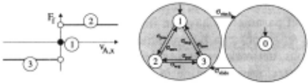
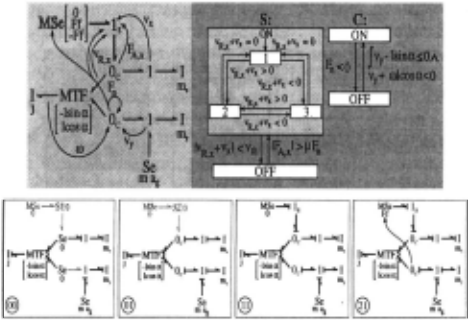
The friction force cannot be predetermined because it depends on the normal force at the surface. When the 0" 3 1ide event becomes active, the friction force comes into effect and its direction is always opposed to the direction of velocity. The events, O"zero, O"po·, and O"neg, correspond to states 1, 2, and 3 of the automata in Fig. 3, respec­ tively. The events that cause these internal state changes are defined as:

Since this behavior is piecewise continuous only simple behavior discontinuities occur at time points, which im­ plies that operational modes have limit values at discon­ tinuities. The complete event set for Coulomb friction is I:= {O"slide, O"·tuck, O"zero, O"po·, O"neg}· A distinction is made between sliding with 0 velocity and being stuck, though the velocity of the rod at the surface is 0. In case the rod is stuck, the model does not have a degree of freedom in the x-direction.

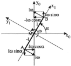
As an example of a transfer of the continuous state vector between model configurations, consider the falling rod when it first makes contact with the floor, the model moves from mode a 00 to mode a 01 in Fig. 5. At this point it reaches a model configuration where Vx and vy at the rod-tip are forced to 0. This requires the center of mass to move in the x and y direction with a velocity that is completely determined by the angular velocity. Conservation of momentum determines that the initial momentum in the y direction is redistributed over the angular and linear momenta. Fig. 2 shows that the linear velocities can be represented in coordinate frame (x0 , y0 ) by Vx = [w+sinB,vy = -[w+cosB. A detailed derivation (see [6]) yields the new state vector:

Figure 4: System state is derived from the original state vector.

3 Model Execution Semantics

A discontinuous change that occurs in given mode ak has to happen at a point in time, say t ·. The state vector at this point, Xak labeled x-;;k = limttt, Xak(t) = Xak(t.). This becomes the a priori vector for the state compu­ tation function g that determines the initial state x+ in the new mode O::k+l· The state vector x+ is referred to as the a posteriori vector computed by g. The new state vector, x+, may immediately trigger further dis­ crete events determined by h and </>, causing a sequence of discrete mode changes till a new operational mode, am, is reached at which no further switching occurs. All the intermediate states traversed between two continu­ ous modes are mythical [7]. The sequence of state and state vector changes is illustrated in Fig. 4. At mode O::m system behavior evolution in time resumes, with the state vector X am (t.) = x+. Sometimes, mode O::m may represent just a point of continuous operation (e.g, the point of contact in an elastic collision [7]) . State vector changes from x-;;k (t.) to x+ in the new real mode may cause the 1 function to generate additional events result­ ing in another sequence of discrete state changes before the next continuous operational mode , an, is arrived at (Fig. 4).

Consider the falling rod in Fig. 5. Initially, it is falling freely under gravity (mode a 00). On hitting the floor it exerts a force with two components, FA,y and FA ,x (mode ao1). Since the floor surface has Coulomb friction, the rod immediately starts to slide if IF A,x I > f.LFn (mode an). Otherwise, it sticks and rotates around the point of contact (mode ao1). When the rod starts to slide, the floor exerts an opposing friction force, F1 . In this case, the initial kinetic energy before contact is redistributed over the angular and vertical momentum to ensure the vertical velocity of the rod-tip, VA,y, is 0. The horizontal velocity of the rod-tip, VA,x, is determined by the angular velocity, w, and the horizontal velocity of the center of mass, Vx. Since Vx is independent of w and determined by FJ, it is initially 0 and the discontinuous change of w results in a discontinuous change of VA ,x · Therefore, the system changes from the operational mode where F1 = 0 to mode 0::21 where F1 = f.LFn.

The grayed modes of operation in Fig. 5 are mythi­ cal. They do not have physical meaning, therefore, no representation on the real time-line. However, they play the role of transition points for locally defined switching functions.

3.1 Temporal Evolution of State

Discontinuities are abrupt point changes, caused by modeling abstractions. Discontinuities that persist in time intervals would violate continuity of power and conservation of energy principles. Further, asymmetry in temporal evolution ensures that the state vector in modes of continuous operation has to be left closed over the time intervals these modes are active. Mode changes and discontinuous changes in the continuous state vec­ tor can only occur at points in time t,. We have shown in other work [7] that further continuous evolution may cause a mode change, am to an, at the point of transfer, but no discontinuous change can occur in the continu­ ous state vector between X am (t,) and xt (t,) since its initial value would be derived from limq.t, X an (t) which requires knowledge of future behavior and conflicts with the assumption of causality in physical system models.

Consider the stiction force when the rod disconnects from the floor as it slides. If this force causes a dis­ continuous change in the vertical velocity of the rod, limq.t , vy (t) differs from the actual value Vy (t,). How­ ever, the value of limq.t, vy(t) may be such that its value indicates that the rod would have gotten stuck. This implies that in addition to the current state vy (t,) and model configuration, the operational mode needs to know future modes and the limit values of state variables looking back in time. Such systems are acausal which is physically impossible and results in ill-defined models.

Since no discontinuous change of the state vector can occur, it is continuous over a left closed interval in time. This only requires the system state to operate continu­ ously in left closed intervals but field f is not required to be differentiable. Therefore, other derived system vari­ ables may still change discontinuously as a result of configuration changes. These jumps are well-defined by the continuous state vector and model configuration.

3.2 Invariance of State

A discontinuous change in the state vector may invoke further mode transitions. The state vector in a new mode is computed from the last continuous state vec­ tor, and the state vector in all new modes is computed from the last continuous state vector before switching started. This is the principle of invariance of state [7] .

To illustrate, consider the falling rod in Fig. 2. When it hits the floor, its vertical momentum is distributed over its angular, horizontal and vertical momentum to ensure its rotation and translation of center of mass are such that the point of contact does not move (mode a 01 ). In this situation, ifthe force at the rod-tip, FA,x, exceeds a threshold value, it immediately starts to slide (mode an). The rod-tip moves freely in the x-direction, and its initial vertical momentum is distributed only over its a posteriori angular momentum and vertical momentum to ensure the y-value does not change at the point of contact. If the continuous state vector in the sliding mode, an, was computed from the previously inferred mode, a 01 , it would have a horizontal velocity associ­ ated with its center of mass which would keep the rod-tip from moving in the x-direction as well, which is incorrect. This demonstrates the importance of the proper compu­ tation of the state vector across a series of discontinuous changes.

3.3 Divergence of Time

Discontinuous configuration changes in system behav­ ior are instantaneous so a model verification technique based on the principle of divergence of time ensures that the model does not end up in a loop of instantaneous changes where system behavior does not progress in time

[7]. In previous work, we have developed a multiple en­ ergy phase space analysis that establishes divergence of time before simulation is performed [5] .

As an example, consider the falling rod when it starts to slide because its force in the vertical direction exceeds a threshold value. If the rod is specified to stick when the velocity of its rod-tip is below a certain threshold value, it may not have sufficient initial vertical momen­ tum to maintain a high enough vertical velocity. Based on the specifications, this moves the model into the con­ figuration where it sticks and rotates around the point of contact. However, in this configuration, based on the initial vertical momentum, its horizontal force causes it to start sliding and a loop of consecutive changes occurs.

3.4 Implementation

In previous work[5; 7], we have developed a hybrid bond graph modeling methodology that uses an ideal switching element, whose on-off conditions are governed by finite state automata, to dynamically construct model config­ urations as its behavior evolves in time. The bond graph model of the idealized thin rod and idealized floor, and the fragments dynamically generated by simulation[6] are shown in Fig. 6. The rod is assumed to have three degrees of freedom with associated buffers: angular ve­ locity w ( buffer J), and linear velocities Vx (buffer mx) and vy (buffer my) . The relation between those veloc­ ities is modeled by a modulated transformer. Gravity is modeled by a constant effort source, mag , in the y direction at the center of mass .

The x and y components of the forces and velocities at point A connect to the model at the Oc junction. If the body is moving freely, this junction is off If the body is in contact with the floor, Oc is on and if no ·other elements are connected, it enforces a 0 velocity. The friction force , FJ = J-tFn, in the x direction is mod­ eled as a piecewise continuous modulated source, M Se, producing force values 0, Ff, -Ff at A opposite to the direction of the surface velocity.

The control specifications (CSPEC) of the switching junctions are specified by finite state automata, one for each controlled junction. The controlled junction is spec­ ified by a hierarchical finite state machine, which can be in one of several on states, depending on the bond graph signals. Depending on the specific state, a part of the piecewise continuous friction function is active. In its off state, the junction enforces 0 flow.

Initially, the rod is moving freely and controlled junc­ tions Oc and ls are off This bond graph is mode goo · The position of the rod-tip closest to the floor , YA , is de­ termined by the sum of the position of the center-point, YM = J Vy , and the distance of the rod-tip from the center point, -lsino:. When XA = 0 the rod collides with the floor, Oc comes on and the model transitions to mode qol· If the rod-length and angle of collision are such that ls comes on (the model transitions into q11) , the rod begins to slide. The function, g, can be recal­ culated, and the piecewise continuous friction function may move into its F1 area, mode q21 . The hybrid bond graph approach provides a seamless integration of con­ figuration changes based on local switches. Details of the derived continuous system and discrete control mod­ els appear in [6]. Other examples of hybrid bond graph models are discussed in [7] .

4 Hybrid System Simulation

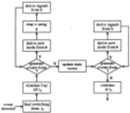
The simulator operates in two modes: (i) continuous simulation during intervals of operation, and (ii) discrete changes during configuration changes. Numerical simu­ lation schemes like Euler and Runge-Kutta can be used for continuous operation but discrete events generated by 'Y triggers an event detection module to determine the switching time, t,, within a margin of tolerance, t. (Fig 7) . The continuous field , /k, computes xk(t;) , then real time is suspended, and the meta-level control model, ¢ , generates the discrete state transition. The original continuous state vector is then transferred to the newly found model configuration using g , and this may trig­ ger further events. The resulting model configuration is established, and Xk (t;) is transferred to this model con­ figuration. Again, discrete events may be generated and this process continues until no further transitions occur and the continuous system state is established as xm(t,)

If the new operational mode is valid for a point in time further events are generated till continuous simulation can be resumed for a model configuration valid over an interval of time. To detect possible configuration changes when the system evolves over an infinitesimal amount of time, the system, fm , is considered continuous over an infinitesimal time, t., i.e., no configuration changes are allowed. Simulation up till t, + t. may cause a new series of configuration changes. These are executed by the discrete model using the h function . There can be no more discontinuous changes so the state vector does not have to be recomputed. In the new continuous mode qn , fn, defines the simulation from timet. with initial vector xm(t.). This implements simulation of fm at t 3 as a point in time and allows an energy redistribution that results from a function with discontinuities that are not simple. Note that the method only applies under the principle of temporal evolution of state.

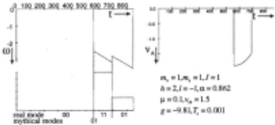
A simulation run for one scenario is shown in Fig. 8. The rod falls down at a specific a,ngle, hits the floor and moves into configuration 01. Based on the state vector an immediate configuration change to mode 11 occurs. In this configuration the rod slides with a velocity that decreases in magnitude due to the friction force acting on the rod-tip. At one time, this velocity falls below a preset threshold value and if the state vector is such that the rod gets stuck without immediately satisfying the condition to slide, the system moves into mode qol· In this mode, it is stuck and rotates around the point of contact until it falls flat on the floor.

5 Conclusions

This work demonstrates a powerful hybrid system mod­ eling scheme that incorporates modeling abstractions and embedded discrete control of physical systems. Con­ figuration changes governed by local automata may pro­ duce discontinuities in system variables. The new state variables are then systematically derived using the prin­ ciple of conservation of state combined with explicitly defined interactions with the environment. Global spec­ ifications are derived dynamically based on systematic principles of invariance of state, divergence of time, and temporal evolution of state. This simplifies the mod­ eling task and truly demonstrates the use of composi­ tionality in defining system models. This is in contrast with the approach by Alur et al. [1] which requires pre­ defined global specifications of continuous system be­ havior in terms of differential equations. Furthermore, global knowledge in specifying discrete behavior is re­ quired to ensure no mythical modes exist . Also, unlike the hybrid bond graph modeling paradigm, there is no support for systematic modeling based on physical prin­ ciples (e.g., conservation of state). The formal speci­ fications are incorporated into a hybrid system simula­ tion scheme that ensures the generation of correct system behavior. Overall, this is a systematic approach to ab­ stracting physical system models: (i) time scale abstrac­ tion, and (ii) ignoring parasitic parameter effects that often cause sharp nonlinearities. The result is a truly hy­ brid behavior generation scheme, where the abstractions result in discrete qualitative behaviors (mode and con­ figuration changes), otherwise system behavior evolves continuously. Future work will be directed toward ap­ plying this methodology in embedded (computer-based) control of physical systems.