Computational and Physical Causality

1 Introduction

In previous work we have discussed how the bond­ graph approach provides a solid basis for the formali­ sation of expert reasoning about physical systems [Top and Akkermans, 1990a; Top and Akkermans, 1990b; Top et a/., 199 Il. It is based on the identification of a small set of physical mechanisms grounded in the energetic aspects of physical systems behaviour: storage processes (storage of energy, capacitor C and inertia I); dissipative processes (resistor R); sources and sinks (Se and Sf); and distribution processes (0- and !-junction, transformer TF and gyrator GY). These mechanisms are represented as nodes in a labelled digraph, linked through energy flows. Thus, the representation embodies energy conservation as a first prin­ ciple of physics. Each energy flow is decomposed into an effort and a flow variable. Each physics domain has its own instantiation of effort and flow variables (for example, force and velocity in mechanics), but the generic notion of effort and flow makes it possible to reason across multiple domains, including mechanics, electrical engineering, hydrodynamics, acoustics and thermodynamics. Thus, bond graphs cover es­ sentially all classical macrophysical domains in an integrated fashion. They are based upon a 'mechanism' ontology. Since the identification of physical mechanisms, which actually are elementary processes, is done on a local basis, this ontology combines attractive features of both the device and process ontologies [Top and Akkermans, 1990b]. It is incorrect to say (e.g. in [Weld, 1990]) that system dynamics (from which the bond-graph method originates) corresponds to the device ontology. The topology of the bond graph can be employed to obtain important qualitative physical information [Top and Akkermans, 1990al Thus, bond graphs provide a formal and generic language for modelling and representing physical systems.

In this paper we will deal with the topic of causality. According to studies of human reasoning about technical devices [Forbus and Gentner, 1986], causal explanations are based on elementary mechanisms that relate individual variables in a directed way. We propose that bond graphs formalise these intuitive ideas in a physically appropriate way, and can be fruitfully employed to obtain causal information based on expert knowledge about physical systems theory. In particular we show that bond-graph causality yields a causal ordering method for physical systems that is similar to but more powerful than the theory of Iwasaki and Simon [Iwasaki and Simon, 1986a].

2 Bond Graph Causality

We will now describe causality from the physical point of view, in terms of bond-graph theory. For an extensive intro­ duction to bond graphs we refer to [Karnopp and Rosenberg, 19751.

2.1 Causality in Physical Systems

Physical models are usually described at a mathematicallevel, where variables are interrelated through mathematical rela­ tions, even if these relations are sometimes called confluences [de Kleer and Brown, 1984] or influences and qualitative pro­ portionalities [Forbus, 1984]. In contrast, bond graphs are based on physical primitives: generic physical mechanisms, linked through energy flows. Causality in bond graphs is rooted in physical intuitions in two ways. First, it is phys­ ically impossible to impose or control both effort and flow simultaneously for a single energy link [Breedveld, 19841. This means that each energy bond defines a bilateral signal flow. In other words, every path of energy exchange is associ­ ated with information flow in both directions along that path. Second, causal directions are constrained by the mechanisms that link individual quantities. This is based on the following physical arguments:

Sources. Sources have fixed causality since they externally impose effort (Se) or flow (Sf). For example, the room atmosphere determines the temperature at the boundary of an experiment, and this temperature is not influenced by the experiment itself. So, the causal direction of bonds connected to sources is determined a priori.

Storage processes. Storage processes have preferred causality. This means that these processes have a priori causal directions at the bonds connected to them, unless the system requires otherwise. A capacitive process prefers to produce effort and an inertial process generates flow, if al­ lowed to. Mathematically speaking, a storage (capacitive or inertial) process defines a relation between one variable and the derivative of another. Although this relation is in itself undirected, in simulations preference is given to causality corresponding to integration rather than differentiation for reasons of numerical stability. This has in itself no meaning for intuitive causality. In [Weld and de Kleer, 1990] Williams concludes from causal explanations given by engineers that 'causality always flows along the direction of integration'. Why this is physically adequate follows from a closer in­ spection of the intuitive understanding of dynamic processes themselves, as we will argue here.

The first argument for integral causality is based on the role that a storage process plays. The 'amounts of stuff' stored by the individual storage processes characterise the present state of a system. These amounts (the state quantities) result from accumulation of flow (or effort). As a result from this accu­ mulation effort (flow) develops. For example, accumulation of liquid due to liquid flow into a container causes the pressure in the container to rise: the state quantity (amount of fluid) is conceived as the cause of the resulting effort (pressure). The reverse statement 'the pressure determines the amount of fluid' is unphysical. Hence, the latter form, corresponding to derivative causality, is avoided if possible; its presence in a model indicates that some dynamic process is (deliberately) being neglected.

The second argument in support of integral causality is based on the fact that causality is conceived as a temporal order of assignment of values. Mathematically, a storage process is represented by q(t) = J; fdr: quantity q is a result of the amount of f that was accumulated over the past period. This is also reflected in the elementary discrete representation of integration: q(t + Llt) = q(t) + f(t)Llt. On the other hand the action of differentiation is intuitively in conflict with causality, since it needs a future value of q: f(t) = ( q(t+Llt)- q(t) )/ Llt. Several mathematical methods have been developed to facilitate numerical differentiation, but these have no physical interpretation.

Resistive processes. Causality at resistive processes is in principle context dependent, i.e., determined by other causal assignments within the model. However, if causality at any such process is not determined by sources or storage processes it remains indeterminate. In that case causality can be assigned indifferently in either of two directions. We will return to this when discussing feedback.

Distribution processes. Distribution processes impose con­ straints on the causal directions of the connected energy­ bonds. A 0-junction must have exactly one effort input, all other bonds generate effort. Consider for example a node in an electrical network: there is only a single voltage level at such a point, imposed from one of the connected lines. On the other hand, a 1-junction may have several input efforts, but has exactly one output effort. Finally, the conversion process TF must have one effort input and one effort output; GY has either effort or flow at both inputs. Since these distribution processes only constrain causal assignment they act as propagators of causality. For instance, if an effort source imposes effort on any of the bonds of a 0-junction, all other bonds must have opposite causality. This in turn may determine causality at other junctions.

2.2 Generation of causal directions

Now we will turn to the generation of causal direc­ tions within a bond-graph model. This is done fol­ lowing the Sequential Causality Assignment Procedure (SCAP) [Karnopp and Rosenberg, 1975; Breedveld, 1986; Rosenberg, 1987] which is one of the most beautiful and powerful tools of the bond-graph method. This procedure is applied to the graph representation of the model and no reference to any mathematical equation is required. Given the local restrictions on causal directions, causality assignment to a complete structure proceeds as follows [Breedveld, 1986]:

1. Choose any source (Se or Sf) and assign its required causality. Propagate the causal implications through the graph as far as possible through distribution processes. Repeat this until all sources have been used.
2. Choose any storage process (C or I) and assign its preferred causality. Propagate causality as far as possible through the distribution processes. Repeat this until all storage processes have been used.
3. Choose any unassigned resistive process (R) and assign arbitrary causality. Propagate causality as far as possible through the distribution processes. Repeat this until all resistive processes have been used.
4. Choose any remaining unassigned bond and assign ar­ bitrary causality. Propagate causality as far as possible through the distribution processes. Repeat this until all bonds have been assigned.

After causality assignment has been completed, which can be the case after any of these four steps, every process math­ ematically represents a directed relation. Thus, propagation of information is completely specified.

2.3 An example

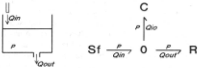
Consider for example the bathtub [Iwasaki, 1988] as shown in Figure 1. The bond-graph model is given on the right. Source of flow Sf represents the incoming flow from the tap, capacitor C represents the storage of fluid in the bathtub and resistor R stands for the action of the outlet. These processes are connected through energy flows to a single 0-junction, representing the fact that they all act on a single pressure P. Energy flows are represented by half arrows, the energy bonds. In the figure it is indicated to which (effort and flow) variables each bond is related at the signal level. Q;0 represents the net flow into the bathtub.

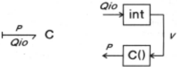
Causality in bond graphs refers to a two-way signal flow. For example, the capacitive process C either must have Q;0 as its input to produce (compute) P as an output or P must be the input and Q;0 the output. If the effort is produced at one side of an energy bond, then flow is produced at the other side. The actual direction of the causal relation is graphically indicated by a causal stroke at the side of effort production. This results in a very elegant and compact representation of causality, as can be seen in Figure 2, for which the associated mathematical decomposition is given on the right in terms of a block diagram. The incoming flow Q;0 is integrated by C to cause an increase of fluid volume V, which causes a rise in pressure P . Note that causal directedness is not restricted to linear systems, as P may depend on V in a non-linear way.

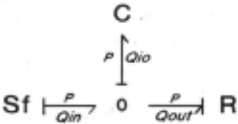
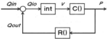
In Figure 3 the bond graph of Figure 1 is augmented with causal directions and Figure 4 shows the equivalent block diagram. The bond graph can be read as follows: At Sf a flow Q;n enters the system. On the other hand, at outlet R flow Q out leaves the system as a consequence of pressure P. The resulting net flow Q; 0 into the container causes an increase of pressure in C.

In order to illustrate how a causal order is generated we use a slightly extended version of the bathtub model. Suppose that the flow is leaving through a long pipe, such that the mass of the fluid contained in it cannot be neglected. This situation is modelled in Figure 5, where I represents the inertial effect of the fluid mass.

According to the above procedure, first causality is assigned to the bond connected to a source of flow. Since this does not yet determine causality at the 0-junction no propagation is possible. Next, effort-producing causality is assigned to the bond connected to C, being one of the storage processes. This immediately determines causality at the 0-junction, which can have only one effort input. The result is shown in Figure 6. No further propagation is possible, because the !-junction is not yet causally determined.

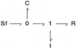
Next, preferred causality is assigned to the bond connected to inertial process I. As a consequence, the !-junction is causally determined (as it can have only one flow input) and the causal direction of the bond connected to R is set. This completes the causal order, since every effort or flow is now an input or an output of some mathematical function, or in other words: it has become a cause or an effect.

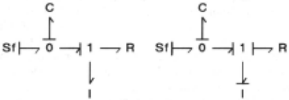
Figure 6: Extended bathtub model after assigning partial and full causality

3 Comparison with the Causal Ordering Theory

The method of causal ordering [Iwasaki and Simon, 1986a; Iwasaki and Simon, 1986b; Iwasaki, 1988; Simon and Rescher, 1966] starts off with a self-contained set of equa­ tions. Exogenous variables are those variables that appear as the only unknown in one of the equations. The values of these variables are substituted in the remaining equations. This re­ sults in some other unknowns being determined, which are said to be caused by the exogenous variables. Next, the newly found values are in turn used to determine other unknowns. This is repeated until all variables are causally ordered.

Causal ordering and bond graphs will produce identical causal order if the underlying mathematical models are equal. From the mathematical point of view a bond graph can be considered as a organisational framework that arranges equations and variables in such a way that substitutions are represented by graphical links, viz., the energybonds. The fundamental difference between both methods is that causal ordering is based on abstract mathematical relations and the bond-graph method on formal physical principles. Thus the causal ordering theory may perhaps also be applied to non­ physical systems. In the realm of physical systems, however, the bond-graph method constitutes a richer representation of knowledge, is better suited for physical explanation, and gen­ erates more causal information. In the following paragraphs this will be elucidated.

3.1 Causal resolution

A causal explanation is acceptable only if (i) the mechanisms on which it is built are intuitively acceptable and (ii) these mechanisms are fully resolved, i.e., two or more mechanisms should not be combined or mixed. That point (i) is satisfied by the bond-graph method has already been discussed in Sec. 1. The second issue points to a problem in the causal ordering theory. Since bond-graphs are based on an exhaustive set of primitive physical mechanisms, they guarantee a maximum causal resolution for a given model 1 . This is not the case for the causal ordering theory. The causal ordering theory does not preclude to produce maximum causal resolution, but leaves it up to the personal skills of the modeller. In contrast, bond graphs generate this as an automated part of the method. For example, in a situation where there is a balance of energy flows in the system, the bond-graph method automatically decomposes this into the mechanisms that create that balance. In the causal ordering theory this decomposition may be easily overlooked by the modeller since it is not necessarily obvious from the mathematical structure of the system.

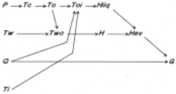
As an example we consider an evaporator as described by Iwasaki and Simon in [Iwasaki and Simon, 1986al Their model consists of 8 unknowns in 8 equations, 4 of which are assumed to be exogenous. The resulting causal order is given in Figure 7. On the other hand, the bond-graph model that is based on the same physical description generates 12 variables and 12 equations (of which 4 are exogenous). The corresponding causal order (Figure 8) shows a much more detailed structure.

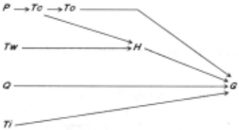
This lack of resolution in the first diagram is partly due to one of their mechanisms (based on the balance of energy flows in the refrigerant) which should have been decomposed further into local mechanisms. As a consequence, the causal order of Figure 7 does not show that Q and T; influence G via Toi · In [Iwasaki and Simon, l986b] a difference variable like To; is called a 'defined' quantity, an artifact of the modelling method that should be avoided since it has no physical meaning. However, every effort (such as temperature or pressure) is defined relative to some reference. Hence, T0 ; is no more an artifact than the so-called 'real' quantities To and T; are. In fact, every effort difference across some path of energy exchange can be the cause of a flow along that path and thus must be considered separately. Consequently, it makes sense to split up H (the total heat absorbed by the refrigerant) into H1;q (heat absorbed by the refrigerant liquid) and Hev (heat absorbed due to evaporation of the refrigerant). For a causal explanation it is definitely relevant to distinguish between all of these quantities.

1 Of course, it is a modelling problem to find out into what detail mechanisms must be distinguished in the real system. However, given a certain detail of modelling it is necessary to preserve that detail in the modelling language.

3.2 Exogeneity

Determining exogeneity is essentially a matter of modelling and certainly not a syntactical issue [Iwasaki and Simon, 1986a]. It is based on assumptions of possible interactions between the system under consideration and the rest of the world. A modeller uses his or her experience and general knowledge of the world to make these assumptions. The theory of causal ordering simply refers to those variables in the system that are not influenced by the system. Bond graphs however provide a more refined approach to exogeneity in the context of physical systems, thus supporting the modeller.

Two types of exogeneity can be distinguished, viz. , direct and indirect exogeneity. Direct exogeneity is related to processes or influences from outside the system that directly determine certain dynamic variables within the system. These influences are represented by sources in a bond graph. In fact, Iwasaki 's suggestion that exogeneity is related to processes which involve 'infinite' amounts of energy [Iwasaki and Simon, l986a] is given a formal basis in the definition of a source. It delivers or consumes energy without being influenced. A battery in an electrical circuit is usually modelled as an ideal source of voltage.

Indirect exogeneity is related to the assumption that a dynamic system is embedded in a fixed structure which is not influenced by the changes of variables. For example, it is usually the case that the capacitance of an electrical capacitor is not influenced by the charge and voltage it is holding (although its value is implied by their values). This type of exogeneity is represented by parameters, to be distinguished from dynamical variables. This physically relevant distinction is usually ignored in AI.

3.3 Self-containment

The theory of causal ordering requires the (static or mixed) mathematical model to be self-contained [Iwasaki, 1988]. It is up to the modeller to check a model and to repair it if does not satisfy tliese requirements: no part of the structure may be overdetermined and the equations may not be dependent. If a model is expressed in terms of a bond graph however, causality assignment automatically checks self-containment. This is due to the fact that after correct causal assignment every variable (effort or flow) is the result of precisely one expression, in which this variable does not occur. The system is said to be in canonical form [Iwasaki, 1988]. Given the initial values at all storage processes a single value for each variable in the system follows.

However, during modelling it is possible to construct a system that is not self-contained. In that case applying SCAP will immediately reveal the problem. For example, suppose we connect two effort sources to a single 0-junction, so that the system is overdetermined. Since a 0-junction cannot accept two efforts as its input, reverse causality has to be assigned for the second source. Hence, a causal error is detected and located. If both effort sources impose equal values one of them is redundant, if they don't the system is inconsistent. This corresponds to the impossibility for two batteries of different voltage and c~nnected in parallel to act like two perfect effort sources.

An interesting application of automatic checking of self­ containment arises if a (mixed) dynamic structure is equi­ librated. Equilibrating refe~ to the process of replacing dynamic mechanisms by thetr corresponding equilibrium mechanisms, in order to find the state of the system after these processes have reached steady-state behaviour [Iwasaki, 1988]. In a bond-graph model equilibrating boils down to replacing capacitive processes by flow sources and inertial processes by effort sources, and setting the respective sources to zero output. Next, SCAP is applied to generate a causal order for the new system. If no causal error is detected the system has a steady-state solution, otherwise the system is overdetermined. In that case simple propagation of values shows whether there is an infinite number of solutions or none [Breedveld, 1984].

3.4 Feedback

In the theory of causal ordering [Iwasaki and Simon, 1986a; Iwasaki and Simon, 1986b] feedback is detected when causal analysis runs into a set of equations that can only be solved simultaneously. The theory does not provide any information about the type of feedback or its sign. Bond graphs in­ corporate a much more clear and informative representation of feedback. Its presence, character and symbolic sign are provided automatically from the causally augmented graph. Moreover, in contrast to the causal ordering theory bond graphs do assign a causal direction within a feedback loop.

Causal loops. A feedback loop within a bond graph simply shows up as a causal loop, i.e., a chain of energybonds with equally directed causality between two storage and/or resistive processes 2 · For example, in Figure 3 the bonds between C, 0 and R represent a causal loop, corresponding to the feedback loop in Figure 4.

2 Any GY within the chain continues it, although the causal direction is reversed.

Only three types of loops are possible. Loops between inertial and capacitive processes introduce two derivatives and thus are of second order (related to oscillation), loops between resistive and storage processes are of first order (related to relaxating behaviour), and loops between resistive processes are static. Hence, the character of a loop can be obtained directly by inspecting the graph.

In general the sign of a feedback loop can be simply derived from the individual directions of the energybonds by tracing the reversals of bond directions within the loop. For example, in Figure 3 the direction of the energy bonds between C and R reverses at the intermediate 0-junction, resulting in a negative feedback loop. In many cases the feedback sign can be found even more easily by applying one of the seven theorems developed in [Brown, 1972].

Thus, the path of a feedback loop, its character, sign and internal causal direction can be established immediately from inspection of the bond graph. However, the net effect of several interacting feedback loops cannot be determined on the basis of qualitative information only, since it depends in a complicated way on the actual values of the parameters. In fact, this points to a basic problem of the Quantity Space [de Kleer and Brown, 1984; Forbus, 1984; Kuipers, 1986]. The resolution of a Quantity Space is too low to allow for an adequate treatment of multiple feedback.

Instantaneous feedback. It may happen that a feedback loop contains no dynamic processes. In that case feedback is mathematically described in terms of a set of simultaneous equations that cannot be solved by simple substitution. Ac­ cording to Iwasaki and Simon [Iwasaki and Simon, 1986b] it is pointless to assign a causal order within such a loop. In the above paragraph we already mentioned that in a bond graph this type of feedback can easily be recognised as a causal loop between two resistive (R) processes. Moreover, the presence of this algebraic feedback is detected already during the application of SCAP: if sources and storage processes do not succeed in determining all causal directions within the model, then the remaining acausal bonds participate in algebraic feedback. As we saw in Section 2, SCAP does not prescribe a preferred causal direction in such a loop. Hence, bond graphs do assign causality within all types of feedback, but in the case of algebraic feedback the direction is arbitrary.

The following argument shows that this agrees with the intuitive conception of causality. An algebraic feedback loop can actually be considered as a dynamic loop that is assumed to reach equilibrium instantaneously, i.e., in a time that is very short compared to the time scale of the rest of the system. However, causal reasoning is only possible in terms of a sequence of causes and effects over time. Since the algebraic loop reaches equilibrium in 'no time' compared to the rest of the system, it makes no difference what comes first. Hence, there is no preferred causal direction. It is interesting to relate this argument to the conclusion in [Iwasaki and Simon, 1986a] that the causal ordering in the equilibrated bathtub example is counterintuitive. Apparently, any causal explanation needs dynamics to be intuitively acceptable. A steady state model is intuitively explained in terms of the associated dynamic behaviour and in a dynamic model (relatively) instantaneous processes are assigned 'virtual' dynamics.

An example of instantaneous feedback can be found in a pressure regulator (see e.g. [de Kleer and Brown, 1984]), between the regulating resistance and the load resistance.

4 Conclusion

It has been argued that the bond-graph method can be fruit­ fully applied to represent and generate causal order in a physical system in a formal way. We have emphasised the physical notions that underly bond-graph causality and have indicated that they conform well with expert physicists' ideas. Assignment of causal directedness is done on a local basis. A causal order is then computationally generated using the sequential causality assignment procedure, applied to the graphical representation of the model.

We have compared this conception of causality with that of the causal ordering theory oflwasaki and Simon [Iwasaki and Simon, 1986al. These two concepts tum out to be similar, but it appears that the causal ordering theory can be put on a firmer physical foundation if it is based on bond-graph causality. It has furthermore been demonstrated, with the help of various examples, that the present approach yields additional causal information. Bond graphs are seen to be more powerful with respect to:

• causal resolution
• exogeneity
• self-containment
• feedback

The causal analysis techniques described in this paper have been fully implemented in QuBA, our system for qualitative bond graph analysis.

Bond graphs constitute a powerful tool for integrated qual­ itative and quantitative analysis of physical systems. This is being strengthened by their application to causal ordering.