
Model-Based Monitoring of Dynamic Systems
Proceedings of the Eleventh International Joint Conference on Artificial Intelligence. Knowledge Representation. Pages 1238-1242.
© 1989 International Joint Conferences on Artificial Intelligence
Abstract
Industrial process plants such as chemical refineries and electric power generation are examples of continuous-variable dynamic systems (CVDS) whose operation is continuously monitored for abnormal behavior. CVDSs pose a challenging diagnostic problem in which values are continuous (not discrete), relatively few parameters are observable, parameter values keep changing, and diagnosis must be performed while the system operates. We present a novel method for monitoring CVDSs which exploits the system's dynamic behavior for diagnostic clues. The key techniques are: modeling the physical system with dynamic qualitative/ quantitative models , inducing diagnostic knowledge from qualitative simulations, continuously comparing observations against fault-model predictions, and incrementally creating and testing multiple-fault hypotheses. The important result is that the diagnosis is refined as the physical system's dynamic behavior is revealed over time .
- [Bratko et al., 1986] Ivan Bratko, Igor Mozetic, and NadaLavrac. Expert Systems: Automating Knowledge Acquisition, chapter Automating synthesis and com- pression of cardiological knowledge. Addison-Wesley, 1986 .
- [Davis , 1984] Randall Davis . Diagnostic reasoning based on structure and behavior. Artificial Intelligence, 24(3) :347-410 , December 1984.
- [de Kleer and Williams, 1987] Johan de Kleer and Brian C. Williams. Diagnosing multiple faults . Artificial Intelligence, 32(1) :97-130, April 1987.
- [Doyle et al. , 1989] R. J. Doyle, S. M. Sellers, and D. J . Atkinson. A focused, context-sensitive approach to monitoring. •In Proceedings of the 1989 International Joint Conference on Artificial Intelligence, August , 1989 . IJCAI
- [Dvorak, 1987] Daniel Dvorak. Expert systems for moni- toring and control. Technical Report AI87-55, Depart- ment of Computer Sciences, The University of Texas at Austin, May 1987.
- [Lee and Dvorak, 1989] Wan-Yik Lee and Daniel Dvo- rak. Learning diagnostic knowledge for dynamic sys- tems. Technical Report AI89-xx (forthcoming), De- partment of Computer Sciences, The University of Texas at Austin.
- [Forbus, 1986] Kenneth D. Forbus. Interpreting mea- surements of physical systems. In Proceedings of the Fifth National Conference on Artificial Intelligence (AAAI-86}, pages 113-117. August 1986.
- [Kuipers, 1986] Benjamin Kuipers. Qualitative Simula- tion. Artificial Intelligence, 29(3):289-338, September 1986.
- [Kuipers and Berleant, 1987] Benjamin Kuipers and Daniel Berleant. Using incomplete quantitative knowledge in qualitative reasoning. In Proceedings of the Seventh National Conference on Artificial Intelli- gence (AAAI-88}, pages 324-329. August 1988.
- [Pearce, 1988] D. A. Pearce. The induction offault diag- nosis systems from qualitative models. In Proceedings of the Seventh National Conference on Artificial In- telligence (AAAI-88}, pages 353-357. August 1988.
- [Perrow, 1984] Charles Perrow . Normal Accidents. Basic Books, Inc., New York, 1984.
- [Quinlan, 1986] J. R. Quinlan. Induction of Decision Trees. Machine Learning, 1:81-106. 1986.
- [Sachs et al., 1986] Paul A. Sachs, Andy M. Paterson, and Michael H. M. Turner . Escort-an expert system for complex operations in real time. Expert Systems, 3(1) :22-29, January 1986.
- [Simmons and Davis, 1987] Reid Simmons and Randall Davis. Generate, test and debug: combining associa- tional rules and causal models. In Proceedings of the Tenth International Joint Conference on Artificial In- telligence (IJCAI-87}, pages 1071-1078. August 1987. IJCAI
References were extracted automatically from the PDF and may contain errors.
Full text extracted automatically from the PDF; figures, tables and equations may differ. The PDF is the version of record.
1 Introduction
Process monitoring is a continuous real-time task of rec ognizing anomalies in the behavior of a dynamic system and identifying the underlying faults. This task is com mon in many industries (e .g., electric power generation, chemical processing, etc.) and in medicine (e .g., cardiac monitoring). In contrast to earlier work on diagnosis, process monitoring poses three special difficulties:
- Diagnosis must be performed while the system oper ates. Process systems are designed for continuous operation and are capable of operating with mul tiple minor faults . Shutdown for diagnosis and re pair is either costly (in industry) or impossible (in medicine) .
*This work has taken place in the Qualitative Reasoning Group at the Artificial Intelligence Laboratory, UT-Austin . Research of the Qualitative Reasoning Group is supported in part by NSF grant IRI-8602665 and by NASA grants NAG 2-507 and NAG 9-200.
tsupported by the AT&T Doctoral Support Program.
Benjamin Kuipers
Department of Computer Sciences The University of Texas at Austin Austin, Texas 78712
r------.,
- Few system parameters are observable. All measure ments come from sensors, which can be expensive and/or unreliable and/or invasive. Monitoring is typically based on a small subset of the system pa rameters, with limited opportunity to probe other parameters.
- The systems are dynamic. The system exhibits time-varying behavior, parameter values vary over a continuous range, the system has state (i.e., has integrated quantities), and feedback is common.
Automated process monitoring systems typically pro vide a set of alarms which are triggered whenever fixed thresholds are exceeded. A nuclear power plant, for ex ample, can have over a thousand distinct alarms, and hundreds of them can be activated within a minute, as in a loss-of-coolant accident. In such situations, process op erators may overlook relevant information, respond too slowly, panic when the rate of information flow is too great , and form incorrect mental models [Perrow, 1984]. The monitoring method described here is intended as an aid to help overcome these problems.
2 Model-based Monitoring
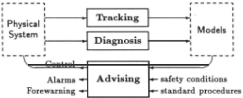
This paper describes MIMIC, a model-based method for monitoring dynamic systems in which the condition of the physical system is represented (and repeatedly up dated) in a dynamic qualitative model. The intent is to mimic the condition of the physical system in the model. Two tasks maintain the model , as shown in Figure 1. The tracking task advances the state of the model in step with observations from the physical system. The diag nosis task, upon identifying a particular fault , injects that fault into the current model so that the predictions of the model will continue to agree with actual observa tions. To be precise, MIMIC maintains a set of candidate models since a given behavior may be caused by one of several faults . Each candidate model represents a possi ble condition of the system (state and faults) .
The purpose of monitoring is to determine the possi ble conditions of the physical system. The role of the advising task is to present this information to the oper ator and assist in interpreting it and making decisions about control actions. Since the models are predictive, they can be used to predict the effect of proposed con trol actions and forewarn of trends leading to undesir able conditions. This paper focuses on the tracking and diagnosis aspects, not on the advising aspect .
2.1 Dynamic Qualitative Models
Two main properties are required of the simulation tech nique used in MIMIC -it must reveal the time-varying (i .e., dynamic) behavior of the system, and it must make explicit the behavioral distinctions important in diagno sis . We use the QsiM [Kuipers, 1986] method for qualita tive simulation of dynamic systems. Just as modern con trol theory represents a dynamic system as a set of cou pled first-order differential equations, QsiM represents a dynamic system as a set of coupled first-order qualita tive differential equations. Simulated dynamic behav ior is represented as a sequence of states, with alternate states representing a time point or time interval in the dynamic behavior .
By using a qualitative model rather than a numeric model, an infinite number of infinitesimally close nu meric behaviors is reduced to a small number of qualita tively distinct behaviors. Although QsiM is fundamen tally qualitative, it can exploit available quantitative in formation to refine its predictions [Kuipers and Berleant , 1987] . This capability proves to be very important in process monitoring because many sensors provide quan t itative values and some faults can only be diagnosed by their subtle-but-quantitatively-noticeable effects .
2.2 Basic Cycle
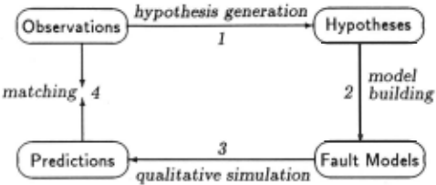
MIMIC accomplishes tracking and diagnosis in a hypothesize-and-match cycle that combines associative and model-based reasoning. In effect , the associative component proposes fault hypotheses and the model based component disposes of them. The cycle has four main steps, as shown in Figure 2:
- Hypothesis Generation. Observations from the physical system may evoke fault hypotheses via a decision tree (the decision tree is generated before hand, as described in section 3). The fault hypothe ses are in the form of specific failure modes (such as a stuck pressure regulator or an abnormal setpoint) and are ordered by likelihood.
- Model Building. Given a combination of one or more fault hypotheses, the corresponding QsiM fault model is instantiated by initializing setpoint variables and mode variables.
- Qualitative Simulation. Each new fault model is first initialized from the observations that evoked its construction, thus establishing the initial state of the model. The model is then simulated incremen tally as observations change, predicting the imme diate successor states. QsiM generates qualitative values and quantitative ranges for each parameter. The ranges may be very precise (e.g. , (98.5 98.7]) or imprecise (e.g. , [0 oo]) depending on the available quantitative knowledge.
- Matching. A similarity function computes the sim ilarity between the observations and a state of the model. The comparison is based on both qualita tive and quantitative values. For similarities above a threshold, the model is retained as a plausible re flection of the physical system's condition. Below the threshold, the model is discarded.
3 Learning Diagnostic Knowledge
The knowledge used in MIMIC's hypothesis generation step is mechanically derived from the model of the dynamic system. The basic technique, as described in [Bratko et al. , 1986], induces fault diagnosis rules from the results of simulating qualitative fault mod els. This technique has been extended to the domain of continuous-variable dynamic systems, as detailed in [Lee and Dvorak, 1989]. Briefly, diagnostic knowledge is derived through five steps:
- Mode/ Definition. A model of the physical system is defined in terms of qualitative differential equations (QDEs) , with some QDEs conditional on the oper ating mode of the component whose behavior they model. For example, a pump will have one set of constraints associated with its normal mode of op eration and another set associated with a "broken" mode.
- Model Building. Using this model definition , a model-building program instantiates the normal (fault-free) model , all single-fault models, and se lected combination-fault models. The issue of which combination-faults to model is discussed in sec tion 4.
- Qualitative Simulation. Using QSIM, each model is simulated starting from each possible initial state, producing a total envisionment for each model.
- Construction of Training Set. Training instances are formed from the states of the total envision-
ment using the qualitative magnitude and qualita tive direction-of-change of each observable param eter. Each instance is tagged with the fault com bination embodied in the model that generated the state. Collectively, these instances form the training set.
- Induction. The training set is compressed by an inductive learning program to a smaller body of op erational diagnostic knowledge in the form of a de cision tree. The induction algorithm is similar to ID3 [Quinlan, 1986], but exploits three additional sources of knowledge: the observability of each pa rameter, the a priori probabilities of faults, and the historical probabilities of behaviors.
The resulting decision tree is used to classify observa tions from the monitored system, yielding fault hypothe ses. The classification procedure ranks the resulting fault hypotheses by likelihood, thus allowing MIMIC to focus attention on the most probable faults. The procedure also produces a ranked set of manually measurable pa rameters whose values, if measured, could reduce the number of hypotheses. MIMIC presents this information to the system operator.
The learning procedure described above can consume a large amount of computer time, but it is performed only once, outside of the real-time monitoring cycle. As Pearce [1988] has demonstrated, this approach to knowledge acquisition provides more complete coverage of faults tharr the traditional knowledge engineering ap proach.
4 Multiple-Fault Diagnosis
The number of fault models that need to be constructed depends on the characteristics of the system being mod eled and the importance of detecting multiple faults. In some domains, single-fault diagnosis is adequate, but in general, multiple faults are common in com plex continuous-running systems. However, complete multiple-fault diagnosis is combinatorially explosive and therefore unrealistic for real-time monitoring of large sys tems. As a middle approach, MIMIC uses a method for incrementally constructing and testing multiple-fault hy potheses. The key ideas are described below.
- MIMIC does continuous monitoring, repeatedly reading the sensors . We assume that faults usually occur one-at-a-time with respect to the sampling rate, so any unpredicted behavior will normally be due to a single additional fault (or a single repair). Thus, MIMIC usually only needs to deal with one new fault at a time.
- Single-fault diagnostic knowledge triggers fault hy potheses whenever any of the manifestations of a sirigle fault are present . Many faults don't interact , so they can be recognized even in the presence of other faults.
- Double-fault diagnostic knowledge captures the manifestations peculiar to every pair of interacting faults . So, if a pair of faults interact in a way that
- obscures either or both of the individual faults, this knowledge can detect both faults.
- The hypothesize-and-match algorithm described earlier is capable of injecting any number of faults into a model. When a fault is hypothesized it may be injected into models that already embody one or more faults . Thus, multiple-fault hypotheses are incrementally constructed and tested.
- Hypotheses are combined in a beam search based on the similarity function described earlier. Let N be the maximum number of models to be tracked, T be the set of models currently being tracked, and F be the newly proposed fault hypotheses. At each cycle then, MIMIC retains the N best models from T U (T x F), ranked by similarity value:
5 Tracking a Model
When a fault model is first constructed, an attempt is made to initialize it from current observations. If the observations are not consistent with any state of the fault model, then the model is discarded. If there is at least one consistent initialization then the model becomes a member of the set of candidate models, and all of its consistent initializations (there may be more than one) are added to the "tracking set" . The tracking set is a set of models, each in a state consistent with the most recent observations.
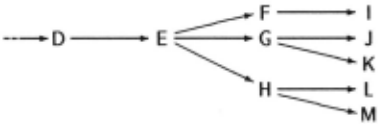
Tracking is the process of using the obser.vations to follow a path through the behavior graph of a model (a "partial envisionment") . Consider the fragment of be·· havior graph in Figure 3. If a model is currently in state E, then a new set of observations is compared (using the similarity function) to the parameter values of state E. If the match is above a threshold, then the model remains in state E. Otherwise, the immediate successor states of state E are generated (via incremental simulation) and each of these states is compared with the observations. If, say, the match with state G was above the threshold, then the model is retained with its state now set to G. If none of the successor states match (up to some limited "distance" from E), then the model is discarded. The limited distance is needed to jump over instantaneous states in the envisionment that fall between consecutive observations.
Observations may include independent parameters, i.e., parameters which are under external control and whose values thus cannot be predicted. When an inde pendent parameter changes value , tracking must reini tialize the states in the tracking set using the current observations and values of history variables (rather than looking in vain for a compatible successor state).
It is possible that tracking could discard all the can didate models . This condition could arise if either: (1) some type of fault was overlooked in the description of possible faults, or (2) the diagnostic knowledge failed to propose one or more faults of a combination fault. In such a case MIMIC (1) alerts the operator that the physical system is behaving abnormally but cannot be diagnosed, and (2) displays the fault hypotheses evoked by the current observations.
6 Example
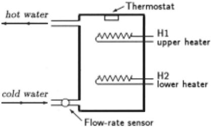
To illustrate MIMIC at work, let's consider the electric water heater shown in Figure 4. It has a single thermo stat which controls whether or not power is applied to the two heating elements (on-off control). Raw sensor information comes from a temperature sensor near the thermostat, from a flow-rate sensor on the cold-water inlet, and from the electric terminals of the heating el ements. In a real monitoring situation we would want to diagnose a variety of possible faults such as defective heating elements, a stuck thermostat, a faulty flow-rate sensor, and loss of electrical power. However, to keep this example simple, we'll consider only the possibility of defective heating elements.
The water heater is modeled in QsiM according to the laws of thermodynamics that relate heat capacity, heat flow, thermal resistance, and temperature. In the normal (fault-free) model all the components of the wa ter heater (tank, heating elements, thermostat, flow-rate sensor) operate according to their intended design. In a fault model, a faulty component operates according to a failure mode (such as a heating element that generates no heat when power is applied).
Table 1 summarizes an example of monitoring the wa ter heater, showing how monitoring progresses over eight moments in a series of observations 1 . For each moment, the table shows the quantitative sensor readings and three sets maintained inside MIMIC. The water heater begins in a state where the water in the tank is hot, the heating elements are off, no water is flowing, and there is a slow temperature loss. These readings are consistent with the normal model. Now, someone starts to draw water for a bath. A high flow rate is measured but all other readings remain the same. Since water flow is an independent variable, MIMIC reinitializes every tracked model (just the normal model in this case) to reflect the change. Since the normal model is consistent with the new values, it is retained.
1 The numeric. values shown in Table 1 are from a numeric simulation of the water heater in which the lower heater is burned out.
As time continues, the temperature inside the tank drops because of the cooler inlet water. These readings are consistent with the current state of the normal model and evoke no fault hypotheses, so no change occurs to the tracking set. At moment 3 the temperature drops to the point where the heating elements turn on (as observed on a voltage sensor), These readings are also consistent with the normal model, so the state of the model is updated accordingly.
At moment 4 the temperature continues to drop. Al though this observation is qualitatively consistent with the normal model, it is inconsistent with the associated quantitative ranges. In effect, the .model is saying that for this flow rate, tank capacity, heating rate, and inlet temperature, the water temperature should not be drop ping so fast. Thus, the tracking task discards the nor mal model. At the same time, the readings are classified by the decision tree as being suggestive of three possi ble faults - a bad upper heating element, a bad lower heating element, or both heating elements bad (denoted bad-H1, bad-H2, and bad-H1,H2) 2 . This causes three fault models to be built. Each model is successfully ini tialized, so MIMIC is now tracking three models.
The water flow stops at moment 5 (somebody turned off the faucet). With this change in an independent pa rameter, MIMIC reinitializes the three models. At mo ment 6, the temperature is observed to be rising. This observation is qualitatively inconsistent with the bad H1,H2 model, so this model is discarded. The observed temperature is then compared to the quantitative predic tions of the two remaining models. Because the observed temperature exceeds the range predicted by the bad-H1 model, that model is discarded. The predictions of the one remaining model, bad-H2, are compatible with the observations, so the model is retained. This model con tinues to track future readings, thus emerging as the sole fault hypothesis.
7 Discussion
The water heater example shows how, with few observ able parameters, MIMIC can diagnose a system by ob serving its dynamic behavior. In general, the speed at which a diagnosis can be narrowed depends on the num ber of monitored parameters and the dynamic activity of the system. With more monitored parameters and more system activity, there are more opportunities to falsify hypotheses.
As a diagnostic method, MIMIC can generate both false positives and false negatives. False positives are common because the relatively small number of ob served parameters cannot, in a single reading, discriminate among all the possible faults . Thus, all but one of the candidates will be a false positive. However, with additional readings that reveal the system's dynamic be havior, the set of candidates can be reduced, sometimes to a single candidate.
2 In a more detailed example, other hypotheses would also be proposed, such as a faulty temperature sensor and a faulty flow meter.
| Moment Synopsis | 0 temp | 1 flow | 2 temp | 3 heater | 4 temp | 5 flow | 6 temp rising | 7 heater off |
|---|---|---|---|---|---|---|---|---|
| hot | starts | dropping | on | still dropping | stops | |||
| Time (min .) | 0.0 | 1.0 | 2.0 | 2.4 | 2.7 | 3.0 | 13.0 | 27.7 |
| Flow (liters/min .) | 0 | 30 | 30 | 30 | 30 | 0 | 0 | 0 |
| Temp. (deg. C) | 64.9 | 64.9 | 61.4 | 58.9 | 57 .1 | 55.9 | 60.0 | 66.0 |
| Power (on or off) | off | off | off | on | on | on | on | off |
| New fault hypotheses | none | none | none | none | bad H1 bad H2 bad H1,H2 | none | none | none |
| New fault model(s) | none | none | none | none | bad H1 bad H2 bad H1,H2 | none | none | none |
| Tracked model(s) | normal | normal | normal | normal | bad H1 bad H2 bad H1 ,H2 | bad H1 bad H2 bad H1 ,H2 | bad H2 | bad H2 |
False negatives can arise either because some type of failure was overlooked in the knowledge acquisition phase or because a combination of three or more faults inter acted in a way that obscured one or more of the indi vidual faults . The former case is solved by adding the new failure type and rerunning the diagnostic learning procedure. The latter case is more difficult. One ap proach is to learn diagnostic knowledge for more than just single and double faults. In the general case this is impractical since the number of fault combinations is exponential in the number of concurrent faults. How ever, in some domains (such as in medicine) the number of realistic combination faults may be tractable because many of the combinations are physiologically impossible or medically uninteresting [Bratko et a/. , 1986].
8 Limitations
MIMIC assumes that faults occur one-at-a-time with re spect to its sampling rate. This assumption may be violated in the case of a catastrophic event (such as an explosion) or cascading faults ; these are real condi tions that MIMIC does not address. Also, MIMIC cannot guarantee that it will recognize any combination faults beyond the combinations included during learning. In practice, it will diagnose many such non-learned com bination faults, but the faults may interact in a way that obscures the manifestations of some subset of those faults .
9 Related Work
Measurement interpretation is a significant part of the job of monitoring, and this aspect of MIMIC shares some of the ideas set forth by Forbus [1986] . In particular, MIMIC's notion of tracking combines two elements of Forbus' approach: that of finding temporally adjacent states in the envisionment which correspond to tempo rally adjacent measurements, and jumping over short gaps where consecutive measurements have missed an intervening instantaneous state in the envisionment .
MIMIC is similar to PREMON [Doyle et a/., 1989] in that both use a qualitative model of the physical sys tem to perform monitoring. However, PREMON is con cerned with monitoring a correctly functioning system in a changing environment. It uses a single fault-free model in a predict-plan-sense cycle for dynamic adjustment of alarm thresholds and for deciding which sensors to fo cus attention on (where the number of sensors is large). This work is complementary to MIMIC's focus on diagno sis, and raises the possibility of combining the techniques to perform diagnostic monitoring on very large systems.
MIMIC differs markedly from model-based trou bleshooters such as GDE [de Kleer and Williams, 1987] in that it (a) uses fault models and (b) does not use de pendency tracing or constraint suspension [Davis, 1984]. Fault models are necessary in MIMIC because of the need to track a faulty system's behavior over time. Faults are specifically modeled (rather than suspending con straints) in order to get reasonably detailed predictions of behavior. Dependency tracing, although extremely useful in domains such as digital logic circuits, provide little diagnostic power in a system of constraints among continuous variables having feedback loops. The prob lem is that dependency tracing in such systems often returns all constraints as suspects because: (a) all pa rameters of a constraint usually affect the result, and (b) output parameters often feed back to input parameters.
The high-level design of MIMIC is similar to the "gen erate, test and debug" (GTD) paradigm [Simmons and Davis, 1987] in that both use associational knowledge to generate plausible hypotheses and model-based reasoning to evaluate them. The core idea in GTD is of "debugging almost right plans" whereas in MIMIC it is of "debugging almost right models".
A number of expert systems have been built which share the same operational goal as MIMIC - that of re lieving some of the burden of monitoring from process operators [Dvorak, 1987]. MIMIC focuses solely on de termining the condition of the physical system, but most of these expert systems have the broader scope of trying to advise the operator on corrective actions. EscoRT [Sachs et al., 1986), an exemplar of this group, gets its knowledge of faults and anomalies and corrective actions through the usual process of codifying human expertise in rules; EscoRT does not encode a predictive model of the physical system as MIMIC does.
10 Implementation Status
Prototypes of MIMIC and its companion learning algo rithm (named DYNALEARN) are implemented in Com mon Lisp and have been run on a Symbolics 3670.
11 Conclusions and Future Work
This paper has presented a technique for online diag nosis (i.e., monitoring) of continuous-variable dynamic systems. The key elements of the design are: (1) repre sentation of continuous-variable dynamic systems in dy namic qualitative/quantitative models, (2) induction of diagnostic knowledge from model simulations, (3) track ing fault-model predictions against observations, and ( 4) incremental creation of multiple-fault hypotheses. The important result is that MIMIC exploits the system's dy namic behavior for diagnostic clues.
Work is progressing on a hemodynamic model of the human cardiovascular system with an expert cardiolo gist . The complete model will have 4 state variables, about 50 parameters, and several regulatory mechanisms (negative feedback loops). As a model of realistic com plexity and scale, this will better reveal limitations of the MIMIC design and areas for improvement.
@inproceedings{ijcai1989p198,
  title     = {Model-Based Monitoring of Dynamic Systems},
  author    = {Dvorak, Daniel and Kuipers, Benjamin},
  booktitle = {Proceedings of the Eleventh International Joint Conference on
               Artificial Intelligence, {IJCAI-89}},
  publisher = {International Joint Conferences on Artificial Intelligence},
  editor    = {N. S. Sridharan},
  pages     = {1238--1242},
  year      = {1989},
  month     = {8},
  note      = {Knowledge Representation},
  url       = {https://ijcai.org/proceedings/1989/198},
}
TY - CPAPER TI - Model-Based Monitoring of Dynamic Systems AU - Dvorak, Daniel AU - Kuipers, Benjamin T2 - Proceedings of the Eleventh International Joint Conference on Artificial Intelligence, IJCAI-89 PB - International Joint Conferences on Artificial Intelligence PY - 1989 SP - 1238 EP - 1242 UR - https://ijcai.org/proceedings/1989/198 ER -Copied
Machine-readable versions of this paper, for tools and AI agents:





