Model-Based Diagnosis using Causal Networks

1 Introduction

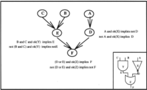
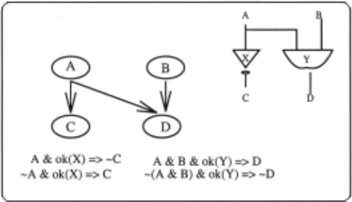
This paper presents an approach for computing diag­ noses [Reiter, 1987; de Kleer et al. , 1992] when the sys­ tem description is structured using a causal network - Figures 1 and 2 depict examples of structured system descriptions.

The most common approach for computing diagnoses has been the use of Assumption-Based Truth Mainte­ nance Systems (ATMSs) [de Kleer, 1986; Reiter and de Kleer, 1987]. We will first explain the difficulties with such an approach and then describe the elements of our approach that address these difficulties.

An ATMS assigns a "label" to each proposition. The label of proposition o characterizes all consistency-based diagnoses of the observation ·o. Once the label of a proposition is computed, one can immediately check whether the proposition is logically true. Therefore, computing labels is no easier than deciding satisfiabil­ ity, which is one source of difficulty with this approach. What makes the ATMS approach especially difficult, however, is that labels can grow exponentially in size, even on very simple diagnostic problems. This difficulty has led to a body of research on "focusing" the ATMS, which attempts to control the size of ATMS labels. Fo­ cusing is based on the following intuition. The label of proposition o characterizes all diagnoses of observation -,o. But one is rarely interested in all diagnoses, there­ fore, one rarely needs a "complete" label. Most often, one is interested in diagnoses that satisfy some prefer­ ence criterion (for example, most probable diagnoses). Therefore, one can use such a criterion to compute "fo­ cused" labels that are of reasonable size, yet are good enough to characterize the diagnoses of interest.

Although a standard framework exists for computing ATMS labels [Forbus and de Kleer , 1993], no such frame­ work seems to exist for focusing.

The approach we present in this paper is based on three main ideas:

Characterizing diagnoses using consequences: We introduce the notion of a consequence for charac­ terizing all consistency-based diagnoses. The size of a consequence (which is a boolean expression) is always less than the size of a label. In fact , there are diagnostic problems that have exponential-size labels and linear­ size consequences.

Utilizing system structure in computing conse­ quences: We introduce a basic algorithm for computing consequences, the complexity of which is parameterized by the topology of the system's causal structure. We show that for singly-connected structures (no undirected cycles), the consequence is always linear in size and can be computed in linear time. For some of these structures, a label can be exponential in size.

A principled mechanism for focusing on pre­ ferred diagnoses: We show that if a consequence has a particular syntax (and-or tree where no symbols are shared between and-branches), then one can extract the diagnoses it characterizes and that meet a specific pref­ erence criterion in time linear in the size of the conse­ quence. Diagnoses with the highest order-of magnitude probability is an example of such a preference criterion.

Therefore, we are providing a paradigm for diag­ nostic reasoning with causal structures, consequences, and preference criteria as the key components. By us­ ing this paradigm, one is guaranteed some complex­ ity results that are parameterized by the topology of the system's causal structure. As we shall see, this approach is based on the causal-network paradigm in the probabilistic and constraint satisfaction literatures [Dechter and Dechter, 1994; Geffner and Pearl, 1987; Dechter and Dechter, 1988]. In both cases , the system structure is the key aspect that decides the difficulty of a reasoning problem. This (conceptually meaningful) pa­ rameter is what diagnostic practitioners need to control in order to ensure an appropriate response time for their applications. The probabilistic literature contains many techniques for tweaking this parameter to ensure certain response times, most of which can be adopted by our proposed framework.

2 Characterizing Diagnoses

In the diagnostic literature [de Kleer et al., 1992], a system is typically characterized by a tuple (.6.,P,A,¢) where .6. is a database constructed from atomic propo­ sitions P U A and ¢ is a sentence constructed from P. The atoms in A are called assumables and those in P are called non-assumables. The intention is that the database describes the system behavior, the assumables represent the modes of system components and the sen­ tence ¢ represents the observed system behavior.

A diagnosis is defined as a conjunction of literals that is consistent with .6. U { ¢} and that includes one literal for each assumable. Therefore, a diagnosis is an assign­ ment of modes to components that is consistent with the system description and its observed behavior. In Figure 1, okX, ok Y and okZ are the assumables and okX 1\ .....,ok Y 1\ okZ is a potential diagnosis.

An ultimate goal of diagnostic reasoning is to com­ pute the most preferred diagnoses (according to some criterion) for a given system (.6., P, A,¢) . The approach we propose in this paper achieves this objective in two steps. First, we compute "the consequence" of observa­ tion ¢, which is a boolean expression that characterizes all the diagnoses of¢. Second, we extract the most pre­ ferred diagnoses from the computed consequence.

The consequence of an observation is defined formally below: 1

Definition 1 The consequence of observation¢, written Cons(¢), is the logically strongest sentence a constructed from atoms A such that .6. U { ¢} f= a. 2

In Figure 2, for example, the consequence · of observa­ tion C 1\ Dis -,okX V -,okY because it is the logically strongest sentence (constructed from assumables) that can be concluded from the given observation and system description.

A consequence characterizes all diagnoses in the fol­ lowing way:

Theorem 1 d is a diagnosis for system ( .6., P, A, 4>) iff d f= Cons(¢).

The consequence -,okX V -,ok Y characterizes three diag­ noses: -,okX f\-,okY, okX f\-,okY and .....,okX 1\okY . Us­ ing "the most probable diagnosis" as the preference crite­ rion, the most preferred diagnoses would be okX 1\ -,ok Y and -,okX 1\okY. We are assuming here that components are unlikely to break, they break independently and their probabilities of failures are equal.

3 The Role of System Structure

We will refer to the triple ( ~, P , A) as a system descrip­ tion and keep it implicit whenever possible. We will also assume that any satisfiable sentence constructed from assumables is consistent with database ~ - This means that the system description does not fix the mode of any component.

Given some observation ¢ and some preference crite­ rion, our ultimate goal is to compute all preferred diag­ noses of ¢ according to this criterion. We will do this in two steps. First, we will compute the consequence of ¢, which characterizes all its diagnoses. Second, we will extract from Cons(¢) the preferred diagnoses. The sec­ ond step will be addressed in Section 5. In this and the following section, we focus on the first step.

We start with the following properties of consequences:

• (C1) Cons(true) =true,
• (C2) Cons(false) =false,

(C3) Cons(¢ V '!f;) = Cons(¢) V Cons( 'I/!), and

• (C4) Cons(¢)= Cons('~/!) when¢= 'lj;.

Note, however, that we do not have Consider the system in Figure 2 for an example. The consequence of C is true, the consequence of D is true, but the consequence of C 1\ Dis -.okX V -.okY.

1 We use a capital letter (sue~ as Y) to denote _an atomic proposition, a small letter (such as y) to denote a literal, and a boldface letter such as Y or y to denote a set of atomic propositions or a set of literals, respectively. ·

2 The consequence of a sentence is unique up to logical equivalence.

If Property C5 were true, then computing conse­ quences would be very easy. To compute the conse­ quence of (, we keep rewriting the expression Cons(() using C1-C5 until we reach a boolean expression that involves only the connectives 1\ and V and consequences Cons('fl), where 11 is an observation that is local to an individual component . Such consequences, called local consequences, can be computed easily since they can be inferred from the component description.

Property C5 does not hold, however, and this makes the computation of consequences more subtle. Prop­ erty C5 may hold in certain cases. When it does, we say that ¢>is "independent" of 1/J. For example, C and D are not independent in Figure 2 because Cons( C 1\ D) :/= Cons( C) 1\ Cons(D) . More generally:

Definition 2 Let I , J , and K be disjoint subsets of P. The sets I and J are conditionally independent given K precisely when

for all conjunctive clauses ex, f3 and 1 over I , J , and K, respectively. 3

When K is empty, we say that I and J are marginally independent . Note that Property C5 is a special case of Property C6 when K is empty since true is the only conjunctive clause over the empty set of atoms.

In Figure 2, for example, let I = { C}, J = { D} and K = {A}. Then I and J are not independent, since Cons( C I\ D) :f= Cons( C) I\ Cons(D) as we verified earlier. However, I and J are independent given K since

and similarly for Cons( C 1\ -.D 1\ A), Cons( -.C 1\ D 1\ A), etc.

Therefore, the key to computing consequences is the ability to detect system independences, which would be used to invoke Property C6. As we shall see next, the causal structure of a system is a very rich source of sys­ tem independences. Explicating such a structure when describing systems, and detecting system independences from such a structure, is the topic of the next section.

3.1 Structured System Descriptions

When a system is described as in Figures 1 and 2, the result is called a structured system description.

A structured system description has two components: A causal structure and a set of component descriptions. The causal structure depicts the interconnections be­ tween system cm;nponents, and component descriptions describe the functionality of system components. 4 For­ mally, a causal structure is a directed acyclic graph, the nodes of which are the non-assumables P . A compo­ nent description is a set of material implications. There is one component description (possibly empty) for each node in the causal structure. The component descrip­ tion associated with node N contains only two types of material implications: 1/J 1\ ex :J N and ¢> 1\ f3 :J -.N, where (1) 1/J and ¢> are constructed from the parents of N in the causal structure; (2) ex and f3 are constructed from assumable atoms A; and (3) 1/J 1\ ex 1\ ¢> 1\ f3 must be inconsistent. These conditions hold iff a component description is local to a single component (1 and 2) and does not constrain the inputs of that component (3).

3 A conjunctive clause over atoms X is a conjunction of literals that includes one literal for each atom in X.

We will use (g, ~, P , A) to denote a structured system description, where g is the causal structure, ~ is the union of component descriptions, P are the atoms in g, and A are the atoms appearing in ~ but not in g.

3.2 System Independences from System Structure

A most important property of a structured system de­ scription is that its topology explicates many system in­ dependences:

Theorem 2 ( [Darwiche, 1993]) Let (9, ~, P, A) be a structured system description and let I , J, and K be dis­ joint sets of atoms in g. If I and J are d-separated by K in g, then I and J are conditionally independent given K wrt to (~,P,A).

d-separation is a topological test that can be performed in polynomial time and is discussed in detail elsewhere [Pearl, 1988].

In Figure 2, { C} and { D} are not d-separated by the empty set, which means that { C} and { D} may not be marginally independent (this was confirmed in the pre­ vious section) . But { C} and { D} are d-separated by {A}, which means that they are conditionally indepen­ dent given {A} .

This independence is useful for computing the conse­ quence of observation C 1\ D. We first use C 1\ D = (C 1\ D 1\ A) V (C 1\ D 1\ -.A) to apply Property C3:

The independence of { C} and { D} given {A} validates Property C6:

Therefore, Cons(C 1\ D)= -.okX V -.okY.

The technique of applying Property C3 to generate consequences that can be decomposed using Property C6 is very powerful. In fact, the algorithm to be given in the following section for computing consequences is based on making (optimal) use of this technique.

4 A structured system description is a special case of a symbolic causal network [Darwiche and Pearl, 1994].

4 Computing Consequences

Before we discuss the algorithm, we will consider a more elaborate example to provide more intuition on the com­ putational value of system independences.

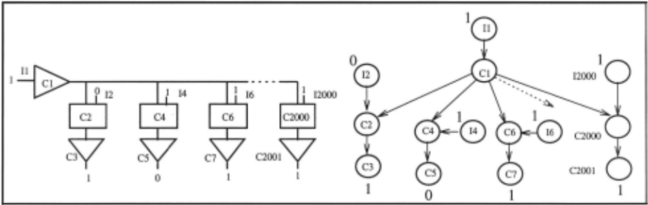
Consider Figure 3, an example from [Freitag and Friedrich, 1992], which depicts part of an audio switch­ ing matrix typically used in broadcasting stations for the flexible connection of studios, recording devices, etc. The given system consists of one input amplifier, 1000 output amplifiers and 1000 switches. For the sake of sim­ plicity, an audio matrix is represented by and-gates and buffers which logically produce the same behavior. The following is observed about the system: the input sig­ nal is ON, the first and-gate gets an OFF signal and all other and-gates get ON signals. The output of buffer C5 is OFF, while outputs of all other buffers are ON. We would like to compute the consequence of this system behavior, therefore, characterizing all diagnoses.

As it turns out, diagnosing this system is easy because its causal structure (shown in Figure 3) explicates inde­ pendences that can be used to decompose the global con­ sequence into local consequences that can be evaluated locally. The systems independences are:

Sll : {h} is independent of all other atoms given {CI}. SI2: {I;,C;,Ci+d are independent of {Ij,Cj,Cj+I} given {CI}, where i,j = 2,4, ... ,2000 and if= j. That is, the atoms corresponding to each connected amplifier and switch are independent of those cor­ responding to other amplifiers and switches given {CI}.

We will now show how these independences can be used to decompose the consequence of interest, Cons(I1 1\ ·h 1\ C3 1\ !4 1\ ·C5 ... I2ooo 1\ C2oo1), which characterizes all diagnoses. The assumables here are abC1, ... , abC2oo1 and the non-assumables are h, h,l4, . .. , hooo and cl, c3, c5, ... , c2001·

We first perform a case analysis on C1 by applying Property C3:

Given Sll, further decomposition is possible using Prop­ erty C6:

Each of the resulting consequences can be evaluated lo­ cally. For example, the consequence of ·C1 1\ h is abC1 and the consequence of cl (\ h is true (normal behav­ ior). Moreover, each of these consequences depends only on the behavior of buffer C1. Similarly, the consequences of C1 1\ ·I2 1\ C3, C1 1\ I4 1\ ·C5 and C1 1\ h 1\ C1 are abC2 V abCs, abC;, V abCs and true, respectively, and these consequences depend only on the behavior of com­ ponents { C2, C3}, { C4 , C5 } and { C6 , C7 }, respectively. Substituting for the above consequences, we get

Cons(I1 1\ ·I2 1\ C3 1\ I4 1\ ·C5 1\ ... hooo 1\ C2oo1)

• = [true 1\ (abC2 V abCs) 1\ (abC4 V abCs) 1\ true 1\ ... 1\true]V

[abC1 1\ (abC2 V abCs) 1\ true 1\ (abC6V abC7) 1\

... 1\ ( abC2ooo V abC2oo1 )],

which simplifies to:

This is the final answer, which is a boolean expression in the form of an and-or tree. This tree will be the input to the focusing phase discussed in Section 5, where the most preferred diagnoses are computed. In the remain­ Cons( C1 1\ ·I2 1\ C3 1\ I4 1\ ·C5 1\ ... I2ooo 1\ C2ooi)] V der of this section, we present the general algorithm for computing c~msequences.

G1ven SI2, we can decompose the above consequences using Property C6:

Cons( C1 1\ ·h 1\ C3 1\ I4 1\ .c5 ... ! 2000 /\ C200I)

• = C (C 1\ I 1\ C ) 1\ C (C 1\ I 1\ C ) ons 1 --, 2 3 ons 1 4 --, 5 . . . Cons( C1 1\ hooo 1\ C2oo1)

Cons( ·C1 1\ ·h 1\ C3 1\ I4 1\ ·C5 ... hooo 1\ C2oo1)

• Cons(·C1 1\ ·h 1\ C3) 1\ Cons(·C1 1\ !4 1\ ·C5) ... Cons(·C1 1\ I2ooo 1\ C2oo1).

1\ C )] The algonthm computes the consequence of observa2001 · tion o , which is a conjunctive clause over a subset 0 of the non-assumables P. The algorithm is symmetric to a well-known one in the probabilistic literature [Pearl, 1988]. It applies to singly-connected networks in which only one undirected path exists between any two nodes. . . The algonthm can be extended to multiply-connected networks in a straightforward manner, leading to an al­ gorithm that is exponential in the size of a network cutset at worse [Pearl, 1988).5

5 Multiply-connected networks are not necessarily harder

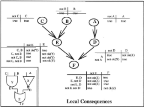
The algorithm works by rewriting the expression Cons( o) using Properties Cl-C6 and stops when every term in the expression is of the form Cons(x 1\ u), where x is a literal of atom X and u is a conjunctive clause over its parents U. The term Cons(x 1\ u) is called a local consequence and it involves a complete observation of all inputs and output of a single component. Figure 4 shows local consequences for the system in Figure 1.

The algorithm can be described as a recursive and deterministic 6 application of the following rewrite rules:

Here, X is an arbitrary node in the network; U and U' are distinct parents of X; Y and Y' are distinct children of X ; and U contains all parents of X. Lowercase letters represent conjunctive clauses over their corresponding atoms.

The algorithm starts by rewriting Cons( o) using Prop­ erty C3 into Cons( x 1\ o) V Cons( ·x 1\ o) for some atom X in the network. To compute the consequence of x 1\ o, the algorithm partitions the observation o into two parts, o_x. about the descendants of X and o1 about the non­ descendants of X ; see Figure 5. This validates Prop-

than singly-connected ones. For example, n-bit adders lead to multiply-connected networks that behave computationally like singly-connected ones.

6 Except for the first rewrite rule, which applies only once.

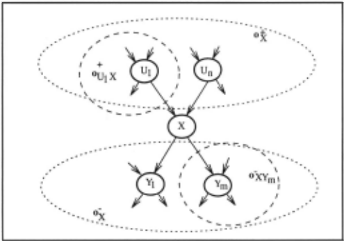
because X d-separates any of its descendants from any of its non-descendants.

To compute the consequence Cons(x 1\ ox) , the algo­ rithm partitions the observation ox into a number of ob­ servations o XY, each about the nodes connected to one child Y of X; see Figure 5. This validates Property C6:

because X d-separates any nodes connected to one of its children from any nodes connected to other children .

To compute Cons(xAoi ), the algorithm applies Prop­ erty C3:

where u is a conjunctive clause over U (the parents of X).

To compute Cons(x Au A oi ), the algorithm parti­ tions the observation o 1 into a number of observations ot x , each about the nodes connected to X through its parent U; see Figure 5. This allows the application of Property C6:

which can also be justified using d-separation and The­ orem 2. A detailed derivation of this algorithm can be found in [Darwiche, 1992].

The complexity of the algorithm is similar to its prob­ abilistic counterpart: linear in the number of arcs but exponential in the number of parents per node. We can verify this by counting the number of conjoin and disjoin operations.

5 Extracting Preferred Diagnoses

The algorithm presented in the previous section com­ putes consequences that have the form of an and-or tree. If component descriptions do not share assumables, then no assumables will be shared by the branches of any and-node in the tree . In this section, we show that if a consequence satisfies the previous two properties, then one can extract from it the most preferred diagnosis in time linear in the size of the consequence, as long as the preference criterion meets some conditions.

The preference criterion is specified by a triple ("E, EB, ~E!)) where "Eisa set of costs, EB is some cost addi­ tion operation and ~EEl is a cost total ordering. 7 The cost function should be such that each literal or its negation has a zero cost and the cost of a diagnosis is obtained by adding the costs of its individual literals. An exam­ ple of such a preference criterion is ( {0, 1, 2, ... }, +, ~), where the cost of a literal is the order-of-magnitude of its probability. 8

Given a preference criterion ("E, EB, ~EEl) and given an and-or tree r (with no assumables shared by branches of and-nodes), one can extract its most preferred diagnoses pd ( r) using the following recursive procedure: 9

1. If r = l , where lis a leaf node, then pd(r) = {l}
2. If r = r1 V r2 , then pd ( r) is the least costly members of pd(r1) U pd(r2) 10

7 EEl is commutative, associative and has a zero element; i~ffij iff i EEl k = j for some k.

8 Note that ([0, 1], *, ;:::) where the cost of a literal is its probability does not satisfy the above conditions since Pr(l) = 1 or Pr(--,/) = 1 does not hold for all literals I!

9 The procedure returns partial diagnoses, which have to be completed using zero cost literals.

10 Properties of the cost function ensure that

It is clear that the above procedure involves only a linear number of recursive calls , one for each node in the tree. What remains to be shown is some guarantee on the size of pd(r;) during these recursive calls. As it turns out, each subtree on which a recursive call may apply repre­ sents the answer to a diagnostic problem that involves part of the observation o and some local observations involving a single component . In particular, each pd(r;) corresponds to one of pd(x A o ), pd(x A oi ), pd(x A ox), pd(x A oxy ), and pd(x A u A otx ), where X is an ar­ bitrary node in the network, Y is one of its children, U is one of its parents, and u is a conjunctive clause over these parents.

We can summarize the guarantees for computing most preferred diagnoses as follows. First, computing the con­ sequence is linear in the number of nodes and exponential in the number of parents per node in a causal structure: The computed consequence has the same size. Second, extracting the most preferred diagnoses from the conse­ quence involves a number of minimization and conjunc­ tion operations that is linear in the size of the conse­ quence. Finally, each one of these operations is applied to a pair of sets, each containing the preferred diagnoses of an asymptotically simpler diagnostic problem.

6 Dual Results for Abduction

There is a dual to consequence calculus, called argument calculus, which associates arguments with sentences in­ stead of consequences. The role that arguments play in abductive reasoning is similar to the role that con­ sequences play in diagnostic reasoning. Following is the definition of an argument wrt a system description (~, P , A) and observation rjJ:

Definition 3 The argument for r/!, written Arg(rfi) , is the logically weakest sentence a constructed from atoms A such that~ U {a} F r/J.

The duality between arguments and consequences 1s given below:

Intuitively, the most general argument supporting rjJ is that the most specific outcome of ·r/J does not hold.

Argument calculus can be viewed as a semantical ATMS since the prime implicants of Arg(rfi) constitute the ATMS label of rjJ [Darwiche, 1993]. This result, to­ gether with Theorem 3, explains the influential role that ATMSs have been playing in diagnostic reasoning.

The following properties hold for arguments [Dar­ wiche, 1993]: A rg( true) = true, A rg(false) = false, Arg(rfi A '!/;) Arg(rfi) A Arg('!f;), and Arg(rfi) Arg('!f;) when rjJ = '!/;. Again, we do not have the prop­ erty: Arg(rjJV'f/;) = Arg(rjJ)VArg('!f;). Consider the system in Figure 1 for an example. The argument for A is false, the argument forD is false, but the argument for A V D is okX.

cost(a)<63cost(,B) only if cost( a 1\ 1)<63cost(,B 1\ 8) for some 1 and all 8 where a 1\ 1 and ,8/\ 8 are conjunctive clauses over assumables.

11 Properties of the and-or tree ensure that cost( a 1\ ,B) = cost( a) EEl cost(,B).

Theorem 4 The sets I and J are independent given K (according to Definition 2} precisely when

(A6} Arg(a V f3 V 1) = Arg(a V 1) V Arg(f3 V 1)

for all disjunctive clauses a, f3 and 1 over I, J, and K, respectively. 12

In Figure 1, { B, C, E} are independent of ( d-separated from) {A, D}. Thus,

Arg(A 1\ B 1\ C :J (·D V E))

• Arg(·A V -.B V -.C V -.D V E)
• A rg( (·A V ·D) V ( -.B V -.C V E))
• Arg( -.A V -.D) V Arg(·B V -.C V E) (using A6)
• Arg(A :J -.D) V Arg(B 1\ C :J E)
• okX V okY.

Given a system description (L\, P, A) and an observa­ tion</;, let us define an abductive diagnosis as a diagnosis o: that (together with the system description) logically entails the observation, L\ U {a} f= ¢;. 13 Then:

Theorem 5 d is an abductive diagnosis of system (L\, P, A,</;) iff d f= Arg(</J).

That is, the argument for observation </; characterizes all its abductive diagnoses. Therefore, Theorem 3 is the basis for a dual set of results for computing abductive diagnoses.

7 Conclusion and Related Work

We have presented an approach for computing the most preferred diagnoses. We formally defined the class of system descriptions and the class of preference criteria to which the approach is applicable. We also characterized the computational guarantees it offers, which we believe are among the sharpest guarantees provided so far.

What is most important about our approach is that it ties the computational complexity of diagnostic rea­ soning to a very meaningful parameter: the topology of a system structure. Thus, it provides diagnostic practi­ tioners with more flexibility in engineering the response time of their applications. This emphasis on structure has been the central theme in probabilistic reasoning lately [Pearl, 1988]. There have been some several at­ tempts to import this theme into model-based diagno­ sis [Dechter and Dechter, 1994; Geffner and Pearl, 1987; Dechter and Dechter, 1988]. A number of structure­ based algorithms have been provided for computing the most likely diagnoses, which seem to have similar compu­ tational complexity and appeal to the same underlying principles. Previous algorithms, however, have rested on the language of constraints among multivalued vari­ ables. A major contribution of this paper is (the sym­ bolic) consequence calculus, which allows computation directly on boolean syntax. This not only simplifies structured-based algorithms significantly, but also pro­ vides a method for humans to compute diagnoses of non­ trivial problems (as illustrated in Section 4).

12 A disjunctive clause over atoms X is a disjunction of literals that includes one literal for each atom in X.

13 An abductive diagnosis of observation ¢>is also called an explanation of¢>.

Another important feature of the presented approach is the very simple and general mechanism for focusing on preferred diagnoses, which comes with useful guaran­ tees. We are unaware of similar guarantees on the com­ putational complexity of focusing using a mechanism as general as the one we have proposed.