
An Inductive Approach to Learning Search Control Rules for Planning
Proceedings of the Thirteenth International Joint Conference on Artificial Intelligence. Machine Learning. Pages 1100-1104.
© 1993 International Joint Conferences on Artificial Intelligence
Abstract
One method for reducing the time required for plan generation is to learn search control rules from experience. Most of the recent work in learning search control knowledge has concentrated on explanationbased learning techniques. An alternative approach is to use inductive learning. An inductive approach does not require a complete and tractable domain theory and has the potential to create more effective rules by learning from more than one example at a time. In this paper, we describe Grasshopper, an inductive system that learns search control rules for a typical plan generation system. We also provide an empirical evaluation of Grasshopper by comparing it with an existing explanation-based learning system.
- [Chien, 1989] S.A. Chien. Using and Refining Simplifica- tions: Explanation-based Learning of Plans in Intractable Domains. In /JCAI-89 Proceedings, pp. 590-595. [Etzioni, 1991] IJCAI
- Etzioni. STATIC: A Problem-Space Com- piler for PRODIGY. In AAAI-91 Proceedings, pp. 533- 540.
- [Fikes and Nilsson, 1971] R.E. Fikes and N.J. Nilsson. S1RIPS: A New Approach to the Application of Theorem Proving to Problem Solving. In Artificial Intelligence 2, pp. 189-208.
- [Gratch and DeJong, 1991] J. Gratch and G. DeJong. A Hybrid Approach to Guaranteed Effective Control Strate- gies. In Proceedings of the Eighth International Workshop on Machine Learning, pp. 509-513.
- [Laird eta/., 1985] J.E. Laird, P.S. Rosenbloom and A. New- ell. Chunking in SOAR: The Anatomy of a General Learning Mechanism. In Machine Learning 1(1), pp. 11- 46.
- [Langley, 1985] P. Langley. Learning to Search: From Weak Methods to Domain-Specific Heuristics. In Cognitive Sci- ence 9, pp. 217-260.
- [Langley and Allen, 1991] P. Langley and J.A. Allen. The Acquisition of Human Planning Expertise. In Proceedings of the Eighth International Workshop on Machine Learn- ing, pp. 80-84.
- [Leckie, 1993] C.A. Leckie. Inductive Learning of Search Control Rules for Planning. Ph.D. Thesis, Dept. of Com- puter Science, Monash University, Australia.
- [Minton, 1988] S. Minton. Quantitative Results Concerning the Utility of Explanation-Based Learning. In AAAI-88 Proceedings, pp. 564-569.
- [Mitchell eta/., 1981] T.M. Mitchell, P.E. Utgoff, B. Nudel and R. Banerji. Learning Problem-Solving Heuristics Through Practice. In /JCAI-81 Proceedings, pp. 127-134. IJCAI
- [Nilsson, 1980] N.J. Nilsson. Principles of Artificial Intelli- gence, Tioga Publishing Corporation.
- [Ohlsson, 1987] S. Ohlsson. Transfer of Training in Proce- dural Learning: A Matter of Conjectures and Refutations? In Computational Models of Learning, L. Bole (ed.), Springer-Verlag, Berlin, pp. 55-88.
- [Quinlan, 1990] J .R. Quinlan. Learning Logical Definitions from Relations. In Machine Learning 5(3), pp. 239-266.
- [Taha, 1975] H.A. Taha. Integer Programming. Theory, Applications, and Computations, Academic Press.
- [Tambe and Rosenbloom, 1989] M. Tambe and P. Rosen- bloom. Eliminating Expensive Chunks by Restricting Expressiveness. ln/JCAI-89 Proceedings, pp. 731-737. IJCAI
References were extracted automatically from the PDF and may contain errors.
Full text extracted automatically from the PDF; figures, tables and equations may differ. The PDF is the version of record.
1 Introduction
The process of generating a plan to satisfy a set of goals can be modelled as a sequence of decisions at different levels of detail. These decisions include choosing which partial solu tion to complete from the available alternatives, which unsatisfied goal to solve next, which planning operator to use in order to attain this goal, and which objects in the domain to use to instantiate this operator. A domain independent planning system uses weak search methods to make these decisions by trial and error. However, by making use of problem solving experience it should be possible to learn domain specific search control rules which reduce inefficien cies in the default search strategy. In this paper, we describe an inductive learning technique for improving the speed of a classical planning system. This technique was implemented in a system called Grasshopper 1 , which learns search control rules to guide the behaviour of a SlRIPS-type planner [Fikes and Nilsson, 1971] within a given domain.
In recent years, explanation-based learning (EBL) tech niques have become the standard approach for this kind of application. For example, systems such as PRODIGY /EBL [Minton, 1988], SOAR [Laird et al., 1985] and STATIC [Etzioni, 1991] all use some variation on EBL in order to increase the efficiency of a planner. However, there can be potential drawbacks to using an explanation-based approach. First, it is a knowledge-intensive method. A domain theory
1 Grasshopper was the name given to the student in the televi sion series "Killlg Fu".
Ingrid Zukerman ·
Department of Computer Science Monash University Clayton, Victoria 3168 AUSTRALIA
Email: ingrid@ bruce.cs.monash.edu.au
is used to prove that a training example is an instance of a particular type of decision. This can pose problems in domains where it is difficult to construct a complete and computationally tractable domain theory [Chien, 1989]. Sec ond, explanation-based approaches learn from a single example at a time. This makes it harder to determine the rel ative importance of each part of a newly learned rule. As a result, additional domain rules or heuristics may need to be encoded to ensure that the new search control rules are stored in an operational form. Otherwise, the cost of testing the applicability of a new rule on future problems may out weigh its savings. This is known as the utility problem [Min ton, 1988].
Grasshopper overcomes these problems by using an inductive approach to learning search control rules for goal, operator and variable binding decisions. Given a number of training instances, the system looks for sets of similar deci sions that could form the basis of new search control rules. It then generates preconditions for these rules by characterising the problem solving contexts in which each of these deci sions occurred. This approach obviates the need to refer to a domain theory, and also improves the utility of new search control rules by taking into consideration more than one training problem when learning a new rule.
In the next section, we describe in more detail the deci sions that arise during planning. In Section 3, we describe our inductive approach. In Section 4, we present the results of testing Grasshopper on several domains using the PROD IGY planner [Minton, 1988], and compare these results with the performance of the PRODIGY/EBL system. These results demonstrate that our inductive approach can produce significant reductions in the time required to generate a plan compared to EBL. In Section 5, we discuss these results and outline issues warranting further research. In Section 6, we outline related work on learning search control knowledge. Throughout this paper, we follow the SlRIPS convention for representing plans and use the "blocks world" domain to illustrate our approach.
2. Search Decisions in Planning
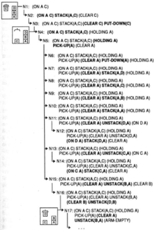
A planning problem is defined by a goal state to be achieved, a starting state from which the goal must be achieved, and a set of operators that can be used to achieve the goal. There are four operators in the standard representation of the blocks world domain [Nilsson, 1980], namely, PUT-DOWN, PICK-UP, STACK and UNSTACK. Figure 1 shows an exam ple of a plan search tree for the top-level goal (ON A C). Each node in the search tree contains a description of the problem state at that node, a goal stack, and a list of the chil dren of that node. As mentioned in the Introduction, at each successive stage in generating a plan the following decisions need to be made.
- Node Decisions: choice of a node containing goals that have yet to be satisfied. In this example, we use the depth-first strategy.
- Goal Decisions: choice of a goal to be satisfied. In this example, it is always the latest sub goal. However, in prob lems where the given goal is a conjunction of simple goals, the choice is important if we are to avoid harmful interactions between the plans for each top-level goal.
- Operator: Decisions: choice of an operator for the cur rent goal. For example, at node NS in Figure 1 there are three different operators which may achieve the goal (CLEAR A): PUT-DOWN, STACK and UNSTACK.
- Binding Decisions: choice of instantiations for the current operator. These are generated by matching the pre conditions of each operator against the current problem state. In situations where there is more than one match, there will be several alternative instantiations of the same operator. For example, UNSTACK is instantiated three times at node NS in Figure 1.
Once all of these decisions have been made, the planner will attempt to generate a new node in the plan search tree. The opportunity for learning in plan generation lies in improving this decision-making process in order to avoid unsuccessful choices.
3. Grasshopper: An Inductive Approach
Grasshopper is designed to analyse a trace of a planning sys tem's behaviour during search, and suggest modifications to the planner's search strategy that will improve its perform ance in the future. Each time the planner solves a problem, the resulting plan search tree is passed to Grasshopper for analysis. Grasshopper then extracts from the plan search tree any interesting decisions that appeared during the search. These decisions are stored and then used as the basis for learning new search control rules. These search control rules are merged with the default rules of the domain to produce a new search strategy that can be used to guide the planner on subsequent problems.
Like PRODIGY/EBL [Minton, 1988]. Grasshopper has been designed to learn about goal, operator and binding deci sions. Grasshopper does not learn about node decisions because any wasted nodes can be explained in terms of the other three kinds of decisions. There are five main stages in Grasshopper:
- First, the Decision Extraction stage extracts interesting planning decisions from a new plan search tree.
- Next, the Decision Clustering stage groups these deci sions according to the type of search control advice they provide.
- The Choice Characterisation stage then learns a unique description for each cluster of decisions. This description is used to recognise when the corresponding advice is applicable.
- The Rule Generation stage compiles the characterisa tion and advice from a cluster of decisions into a search control rule. This may result in a new rule, or an updated version of an existing rule.
- Finally, the Utility Optimisation stage estimates the utility of new rules, and decides whether they should be passed on to the planner.
In the following subsections, we describe the operation of each of these five stages. Since the same basic approach is used for the three kinds of planning decisions, we focus on learning about operator decisions, and describe any major deviations from this method where appropriate. For a more detailed description of Grasshopper, see [Leckie, 1993].
3.1 Decision Extraction
When Grasshopper is given a new plan search tree, its first task is to extract interesting decisions for learning. This is done by applying two basic guidelines: (1) do not attempt to learn from a decision if all of its choices have been doomed to failure by an incorrect choice at a higher level decision, and (2) do not attempt to learn from a decision if there was only one possible choice. In other words, Grasshopper is interes~d in decisions where there is more than one choice available, and one of those choices eventually led to a suc cessful plan.
The first guideline forces Grasshopper to filter out nodes that are not ancestors of the successful leaf node of the plan search tree. Given a successful leaf node for a plan, it is a simple matter to trace its ancestors back up to the root of the tree. We refer to the successful leaf node and its ancestors as the successful nodes of the plan. For example, in the problem in Figure 1, the successful nodes are {N1, N2, N3, N4, NS, N15, N16, N17, ... }.In contrast, nodes N6 to N14 contain no decisions with successful choices because they are all derived from incorrect operator or binding choices at node NS. Consequently, they are excluded by Grasshopper.
Grasshopper then applies the second guideline in order to find interesting examples of each kind of planning decision from each of the successful nodes in the plan. For example, there is only one possible operator choice for the goal (ON A C) at node N1 in Figure 1. Consequently, node N1 is excluded by the second guideline. In contrast, there are sev eral possible operator choices for the goal CLEAR. Conse quently, nodes N2, NS and N15 are all extracted as ex~ples of interesting operator decisions. The same procedure ts used to extract examples of goal and binding decisions. Clearly, there are no interesting examples of goal interactions in Fig ure 1 because the problem involves only one top-level goal.
3.2 Decision Clustering
Once Grasshopper has extracted the interesting examples of each kind of decision, it needs to cluster these decisions according to the type of advice they provide. Interesting decisions are organised into a data structure known as a choice table. Separate choice tables of each kind of planning decision are maintained in Grasshopper as a long-term mem ory. A choice table clusters decisions using two levels of indexes. At the first level, decisions are indexed according to their decision type. For example, operator decisions have the same decision type if they all involve the same kind of goal. Consequently, nodes N2, NS and Nl5 from Figure 1 would all be indexed under the decision type CLEAR. At the second level, decisions of the same decision type are sub-indexed according to their choice type. For example, operator deci sions have the same choice type if they all have the same operator as their successful choice. Consequently, the deci sion type for the goal CLEAR would be sub-indexed so that node N2 is stored under the choice type PUT-DOWN, while NS and Nl5 are stored under the choice type UNSTACK.
The same procedure is followed for goal and binding decisions. In the case of goal decisions, the decision type is defined by the predicates of the interacting pair of goals, while the choice type is the goal that avoids harmful interac tions when satisfied first. In the case of binding decisions, the decision type is defined by the goal predicate and opera tor type for the decision, while the choice type denotes whether or not the chosen list of bindings was successful. Grasshopper has to store unsuccessful binding decisions so that it has a supply of counter-examples for learning. This is not necessary for goal and operator decisions, where the counter-examples of a choice type are implicit in the other choice types belonging to the same decision type.
The choice types indexed under the same decision type represent competing choices for the same type of decision. Clustering decisions in this way structures the learning prob lem for Grasshopper, since each choice type represents an opportunity for a search control rule.
3.3 Choice Characterisation
Each successful choice type in a choice table represents a target concept for learning. Before Grasshopper can encode a rule for such a choice type, it needs to characterise when that advice is applicable. Sometimes the choice is clear, such as when one type of goal is always preferred to another. For other decision types the correct choice may not be so obvi ous, such as when two successful choice types have been observed for the same decision type. In this case, the correct choice depends on the context of the current decision. The role of the Choice Characterisation stage is to learn a gener alised description of the decision context that discriminates the correct choice for a decision from any distractors.
For example, we saw in the last subsection that the deci sion type CLEAR has at least two choice types, i.e., PUT DOWN and UNSTACK. In other words, in some situations PUT-DOWN is the correct choice, while in other situations the planner should use UNSTACK. The difference bet~~en these two situations is the problem state where each dectsiOn was made. Consequently, if Grasshopper is to generate a search control rule for each of these choice types, it needs to encode into the rule the problem state features that discrimi nate one situation from the other. Specifically, each choice type must be discriminated from every other choice type of the same decision type. This involves searching for a gener alised problem state deseription that matches all the deci sions in the target choice type, and none of the decisions in any of the competing choice types.
We have adapted the FOIL learning algorithm [Quinlan, 1990] to perform this task. FOIL learns an intensional defini tion for a target relation that is given as a set of positive and negative examples. This definition is represented as a set of Hom clauses that define the target relation in terms of a set of background relations. These Hom clauses are constructed so that between them they match all the positive examples of the target relation without matching any of the negative examples. FOIL uses an information-based heuristic to guide a greedy search for the relations to be used in the body of each clause. Interested readers are referred to [Quinlan, 1990] for a detailed description of the operation of FOIL.
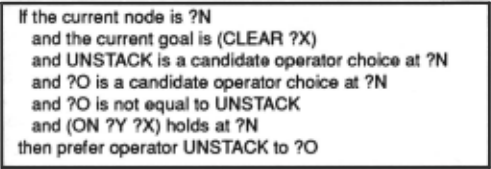
In our application, the target relation is the choice type to be characterised and the background relations encode the context of the decision. Consider the problem of characteris ing the choice of the operator UNSTACK for the goal CLEAR. The target relation contains two positive examples, corresponding to the operator decisions at nodes NS and Nl5, and one negative example, corresponding to the node N2. The background relations encode the goal predicate and the current problem state for each of these examples. Using the FOIL algorithm, Grasshopper finds that the feature (ON ?Y ?X) is unique to decisions where UNSTACK is successful for the goal (CLEAR ?X). Similarly, Grasshopper finds that the feature (HOLDING ?X) is unique to decisions where PUT DOWN is successful for this goal.
Each clause that Grasshopper learns in this way forms the basis for a new search control rule. The main advantage of using a learning algorithm such as FOIL is that it provides an efficient method for characterising each choice type. In addi tion, it is able to learn about choice types that require a dis junctive description, i.e., choice types that cannot be characterised by a single clause.
3.4 Rule Generation
Once interesting decisions have been clustered and charac terised, the Rule Generation stage can begin. Rules are required only for those choice types that have been confused with alternative choices of the same decision type. The resulting rules may then be used by the planner to avoid making the wrong choice in subsequent problem solving.
For each choice type that requires a rule, Grasshopper needs to encode the antecedent and the consequent of the rule. The antecedent encodes the context of the decision. This is used by the planner to recognise whether the rule is applicable at a given node in a plan search tree. It specifies the decision type, the competing candidate choices, and the characteristic features of the successful choice type. The consequent of a rule encodes the advice contained in the choice type. One approach is to encode this advice so that the successful choice is the only available option for the planner. However, this may lead to the correct choice being pruned from the search space if the characterisation used in the rule is too general. Consequently, Grasshopper encodes the advice of a rule as a preference for the successful choice type over the other candidate choices. Figure 2 illustrates an example of such a search control rule.
3.5 Utility Optimisation
Any choice type in the choice table that contained erroneous choices before the successful choice was found may warrant a rule. Such a rule saves the cost of repeating these mistakes in the future. However, there is an overhead to adding new rules. Every time a node is expanded, we incur the cost of testing this rule. If the savings of the rule are small, or if the rule is seldom applicable, then the utility of the rule to the planner is low. Hence, we need to estimate the utility of new rules before they are added to the planner.
We can calculate a measure of this utility using the infor mation collected from the training problems as they appear in the choice table. We begin by calculating the cost of solv ing each training problem. This is just the cost of creating the nodes in the search tree. A search control rule would reduce this cost by the number of wasted nodes that it would save from the training examples, e.g., nodes N6-N14 in Figure 1. In return, there would be an additional overhead of matching the rule at every node in the tree, excluding the nodes that have been saved. When this process is repeated for every choice type in all three choice tables, the expression for the total choice cost is as follows:

where:
t = total number of choice types, n. = number of decisions represented by choice type i, ~- = number of wasted nodes in decisions of choice type i, x .' e { o, 1 } 1 if the rules for choice type i are included, I · 0 otherwise, C = average cost of creating a node, and c c = average cost of matching a rule to a node. m Note that in order to simplify this calculation, we have used average values for the costs of matching rules and cre ating nodes.
We use this approximate expression to help quantify the effect that new candidate rules would have on the training problems. The problem of determining which rules to remember can thus be resolved by finding the combination of rules that minimise this cost function. Unfortunately, how ever, in order to calculate the additional overhead of any par ticular rule, we need to know which other rules have been included. As a result, the optimisation of this cost function is a non-linear 0-1 integer programming problem [Taha, 1975]. There are 2' possible alternatives in the search space for such a problem. However, in all of the domains we have encountered, t is sufficiently small to allow us to perform the search using explicit enumeration.
4. Experimental Results
In this section, we examine the performance of Grasshopper in practice, using the PRODIGY planner as our test-bed. The performance of Grasshopper was compared with two alter native strategies. The first alternative was the default search strategy used by PRODIGY. The other alternative was the search strategy learned by PRODIGY /EBL, which has become a standard example of the state of the art in EBL. Our aim is to compare the utility of our inductive learning approach to that of EBL.
Our inductive algorithm has been tested in four domains, three of which we present in this section. The first two domains are the versions of the blocks world and STRIPS world used in [Minton, 1988]. In each case, a training phase of 50 problems was followed by a testing phase of 100 prob lems. The problems were randomly generated and varied in complexity from one to five goals. The training problems were filtered to exclude examples that were too hard or too easy. The third domain implements a parser for strings of the ambiguous grammar shown in Figure 3. This simple domain is included to illustrate the advantages of inductive learning when a problematic domain theory is involved. In this case, a training phase of 10 problems was sufficient to learn appro priate search control rules. It was followed by a testing phase of 50 problems.
In the first and third experiments, the length of the search on each problem was limited to a maximum of either 300 CPU seconds or 2500 nodes, whichever came first. In the STRIPS world domain, the CPU bound was raised to 750 seconds so that at least one strategy was able to solve all of the test problems. The tests were run on a Sun Sparcstation IPC using Sun Common Lisp 3.0. It should be noted that detect any significant patterns. However, Grasshopper was PRODIGY /EBL was able to create search control rules for able to achieve its level of performance · using the same node decisions in addition to goal, operator and binding number of training examples used by PRODIGY /EBL. The decisions. Further, in the blocks world and S1RIPS world only noticable difference was that PRODIGY /EBL usually domains, PRODIGY /EBL had access to explicitly encoded required less time for learning than Grasshopper. The largest domain axioms that could be used to help simplify the expla- difference observed was a factor of approximately two in the nations that were generated. S1RIPS world domain.
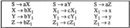
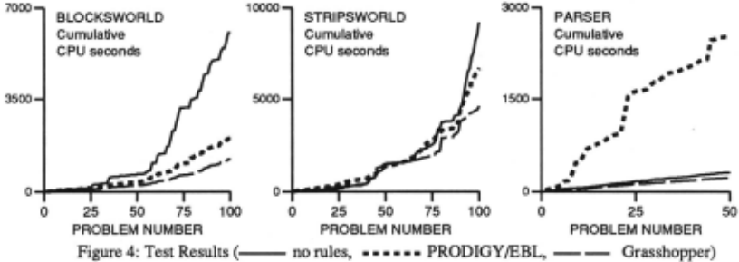
The results of these tests are plotted in Figure 4. These Another advantage of domain theories is that it is possible graphs show the cumulative cost of the search in terms of the to verify the correctness of the rules that are learned. For CPU time spent on each problem. According to these results, example, some characterisations learned by Grasshopper the rules learned by Grasshopper were most effective at were initially too specific or too general. However, most of reducing the total search time required in all of the domains. these errors were eliminated by the end of the training phase, In terms of the total number of nodes expanded, there was since Grasshopper relearns a rule if it sees a new example. little difference between Grasshopper and PRODIGY /EBL Those errors that persisted still led to rules that were useful in the blocks world and parser domains. In the S1RIPS part of the time, even though they gave the wrong advice on world domain, PRODIGY /EBL produced greater savings in some occasions. In contrast, correctness does not guarantee the number of nodes expanded, as shown in Table 1. How- utility. For example, although the rules learned by PRODever, PRODIGY /EBL required more rules than Grasshopper IGY /EBL in the parser domain were correct, they were far to achieve these savings. This means that these savings were too complex to be useful because of the recursive nature of offset by the additional computational cost of having to test a the domain theory. Grasshopper was able to learn much simlarger set of rules at the nodes of each search tree. Thus, the pier rules because it tested for the feature that characterised utility of the rules learned using the inductive approach is each string, namely, whether it contained the letter "x", "y" significantly higher than that of the rules learned using the or "z". Although this is an artificial domain, it illustrates the explanation-based approach. ability of inductive techniques to learn from heuristic fea tures that are hard to explain or not mentioned in the domain 5. Discussion and Further Work theory. An interesting issue for further research is to study these kinds of domains in more detail.
Our results have demonstrated the advantages of inductive learning in addressing the utility problem. By learning from more than one example at a time, it is possible to avoid learning rules that are overly specialised to individual exam ples. This raises several issues regarding the role of a domain theory in learning search control knowledge. An advantage of using a domain theory in explanation-based learning is that it provides a strong bias in the search for a set of features that characterise a target concept. This reduces the number of training examples required for learning. Consequently, it is often a criticism of inductive learning techniques that they may require a large number of examples before they can Finally, our cost function was able to provide an efficient test of the utility of the rules learned by Grasshopper. In these three domains, all of the rules that were learned by Grasshopper were deemed to be useful and passed on to the planner. The performance of these rules in practice supports this decision. An issue for further testing is to repeat these tests using subsets of the final set of rules in order to deter mine whether there were any errors of commission.
| Strategy | Active Rules | Nodes Expanded | Unsolved Problems |
|---|---|---|---|
| Detault | - | 37174 | 7 |
| Grasshopper | 14 | 10145 | 0 |
| PRODIGY /EBL | 29 | 2708 | 1 |
6. Related Work
The current trend in learning search control knowledge to reduce the cost of planning has been towards EBL. So far, we have concentrated on PRODIGY/EBL. Other explana tion-based systems that address the utility problem are SOAR [Tambe and Rosenbloom, 1989] and STATIC [Etzi oni, 1991]. SOAR uses a technique known as "chunking" to learn search control knowledge from experience. It avoids the problem of expensive chunks by restricting the ways in which domains can be encoded. STATIC takes a different approach by learning search control rules from the domain definition only, without referring to training examples. It avoids expensive rules by excluding rules that require a recursive proof. Both of these approaches to intractable domain theories have the effect of restricting the range of concepts that can be learned. In contrast, Grasshopper can learn heuristic features that are not amenable to explanation. In addition, neither of these systems attempts to evaluate the utility of the knowledge that is learned, unlike Grasshopper and PRODIGY /EBL.
There are a number of systems that have used inductive techniques to learn search control knowledge. Early systems, such as LEX [Mitchell eta/., 1981], SAGE [Langley, 1985] and UPL [Ohlsson, 1987] learned search control rules to guide problem-solvers that use production rules. Unlike Grasshopper, these systems were not designed to work with a planning system. Consequently, they did not attempt to learn about goal interactions. In addition, these systems were developed before the utility problem became a major issue. As a result, they did not investigate the utility of the knowl edge learned using inductive methods. More recently, unsu pervised inductive learning has been used in a system called DAEDALUS [Langley and Allen, 1991] to learn concept hierarchies that can guide a planner. These concept hierar chies are used to provide advice on planning decisions by recalling the choices that were made in similar situations in tht': past. In terms of utility, the process of matching a new decision against a concept hierarchy is a significant compu tational overhead. However, their main concern is with cog nitive issues, rather than with the utility problem.
Finally, COMPOSER [Gratch and DeJong, 1991] uses a similar approach to our own for estimating the utility of rules in combination. Their approach is more elaborate, in that they model how the savings of a rule change when other rules are added. In addition, they use statistical tests to deter mine upper and lower bounds on the utility of a set of rules, and use a greedy strategy for selecting rules. The trade-off of using a more elaborate model is that COMPOSER may need more training examples than Grasshopper in order to satisfy the statistical tests. In addition, COMPOSER requires extra time for plan generation during the training phase so that it can measure the match cost of rules before they are added. An issue for further study is whether a more elaborate model such as this leads to significant improvements in utility, or whether there is a diminishing return due to increased train ing time in practice.
7. Conclusions
In this paper, we have addressed the problem of how to improve the speed of a planning system by learning from experience. Specifically, we have developed and tested an inductive learning algorithm which generates search control rules for goal, operator and binding decisions in planning. Unlike EBL methods, this approach can generate rules of high utility without the need for additional domain knowl edge or heuristics to indicate which domain features are rele vant to a rule. In addition, we have presented a new method for estimating the utility of learned rules by studying the effect of new rules in combination on the performance of the planner. We have demonstrated in three test domains that our approach can significantly reduce plan search time in com parison to an explanation-based system.
8. Acknowledgements
The permission of the Director, Telecom Research Laborato ries, to publish this paper is hereby acknowledged. We are extremely grateful to the PRODIGY team at Carnegie Mel lon University for providing us with a copy of their system.
9. References
[Chien, 1989] S.A. Chien. Using and Refining Simplifica tions: Explanation-based Learning of Plans in Intractable Domains. In /JCAI-89 Proceedings, pp. 590-595.
[Etzioni, 1991] 0. Etzioni. STATIC: A Problem-Space Com piler for PRODIGY. In AAAI-91 Proceedings, pp. 533540.
[Fikes and Nilsson, 1971] R.E. Fikes and N.J. Nilsson. S1RIPS: A New Approach to the Application of Theorem Proving to Problem Solving. In Artificial Intelligence 2, pp. 189-208.
[Gratch and DeJong, 1991] J. Gratch and G. DeJong. A Hybrid Approach to Guaranteed Effective Control Strate gies. In Proceedings of the Eighth International Workshop on Machine Learning, pp. 509-513.
[Laird eta/., 1985] J.E. Laird, P.S. Rosenbloom and A. New ell. Chunking in SOAR: The Anatomy of a General Learning Mechanism. In Machine Learning 1(1), pp. 1146.
[Langley, 1985] P. Langley. Learning to Search: From Weak Methods to Domain-Specific Heuristics. In Cognitive Sci ence 9, pp. 217-260.
[Langley and Allen, 1991] P. Langley and J.A. Allen. The Acquisition of Human Planning Expertise. In Proceedings of the Eighth International Workshop on Machine Learn ing, pp. 80-84.
[Leckie, 1993] C.A. Leckie. Inductive Learning of Search Control Rules for Planning. Ph.D. Thesis, Dept. of Com puter Science, Monash University, Australia.
[Minton, 1988] S. Minton. Quantitative Results Concerning the Utility of Explanation-Based Learning. In AAAI-88 Proceedings, pp. 564-569.
[Mitchell eta/., 1981] T.M. Mitchell, P.E. Utgoff, B. Nudel and R. Banerji. Learning Problem-Solving Heuristics Through Practice. In /JCAI-81 Proceedings, pp. 127-134.
[Nilsson, 1980] N.J. Nilsson. Principles of Artificial Intelli gence, Tioga Publishing Corporation.
[Ohlsson, 1987] S. Ohlsson. Transfer of Training in Proce dural Learning: A Matter of Conjectures and Refutations? In Computational Models of Learning, L. Bole (ed.), Springer-Verlag, Berlin, pp. 55-88.
[Quinlan, 1990] J .R. Quinlan. Learning Logical Definitions from Relations. In Machine Learning 5(3), pp. 239-266.
[Taha, 1975] H.A. Taha. Integer Programming. Theory, Applications, and Computations, Academic Press.
[Tambe and Rosenbloom, 1989] M. Tambe and P. Rosen bloom. Eliminating Expensive Chunks by Restricting Expressiveness. ln/JCAI-89 Proceedings, pp. 731-737.
@inproceedings{ijcai1993p152,
  title     = {An Inductive Approach to Learning Search Control Rules for Planning},
  author    = {Leckie, Christopher and Zukerman, Ingrid},
  booktitle = {Proceedings of the Thirteenth International Joint Conference on
               Artificial Intelligence, {IJCAI-93}},
  publisher = {International Joint Conferences on Artificial Intelligence},
  editor    = {Ruzena Bajcsy},
  pages     = {1100--1104},
  year      = {1993},
  note      = {Machine Learning},
  url       = {https://ijcai.org/proceedings/1993/152},
}
TY - CPAPER TI - An Inductive Approach to Learning Search Control Rules for Planning AU - Leckie, Christopher AU - Zukerman, Ingrid T2 - Proceedings of the Thirteenth International Joint Conference on Artificial Intelligence, IJCAI-93 PB - International Joint Conferences on Artificial Intelligence PY - 1993 SP - 1100 EP - 1104 UR - https://ijcai.org/proceedings/1993/152 ER -Copied
Machine-readable versions of this paper, for tools and AI agents:





