First Results in Robot Road-Following

First Results in Robot Road-Following

Richard Wallace, Anthony Stentz Charles Thorpe, Hans Moravec William Whittaker, Takeo Kanade

Robotics Institute, Carnegie-Mellon University

Abstract

The new Carnegie-Mellon Autonomaus Land Vehicle group has produced the first demenstratians of road-following robots. in this paper we first describe the robots that are part of the CMU Autonomaus Land Vehicle project. We next describe the vision systern of the CMU AL V. We then present the control algorithms, inc!uding a simple and stable control scheme for visual servoing. Finally, we discuss our plans for the future.

Jntroduction

CMU has formed the Autonomaus Land Vehicle (AL V) group to develop a perceptive outdoor robot. We have produced the first demenstratians of an autonomaus vehicle able to follow a road using a single on board black and white television camera as its only ser.sor. Our robot has made several successful runs over a curving 20 meter path, and 10 meter segments of staright sidewalk, moving continuously at slow speeds, by tracking the edges of the road.

The research described in this paper is a first complete system, covering everything from low-level motor drivers to the top-level control loop and user interface. We took a "depth-first" approach to building our testbed: we picked one rough design and built all the pieces of a functioning system, rather than spending a Iot of time at the beginning exploring desi"gn alternatives.

Related research at the Unversity of Maryland [6] has focused on the problern of visually finding and tracking roadways. The "bootstrapping" phase of the Maryland road finding program, in which the robot detects a road on start-up with no a priori position information, currently has no counterpart in our system. Our vehicle is always started with an orientation rnore or less aligned with the direction of the road and with knowledge of an initial road model. The Maryland road finding module is expected to be tested soon on an AL V built at Martin Marietta Denver Aerospace.

ln this paper we first describe the robots that are part of the CMU Autonomaus Land Vehicle project. We next describe the vision system of the CMU AL V. We then present the control algorithms, including a simple and stable control scheme for visual servoing. Finally, we discuss our plans for the future.

Currently, this prnject is funded in part by Carnegie-Mellon University, by the Office of Naval Research under contract nurnber N00014-81-K-0503, by the Western Pennsylvania Advanced T echnology Center. by Defense Advanced Research Projects Agency (DOD). ARPA Order No. 3597, monitared by the Air Force Avionics Labaratory under contract F3361~·81-K-1539, and by Denning Mobile Robotics, lnc. Hochard Wallace th3nks NASA for supporting him with a NASA Graduale Student Researchcrs Program Fellowship Grant.

Terregator and Neptune

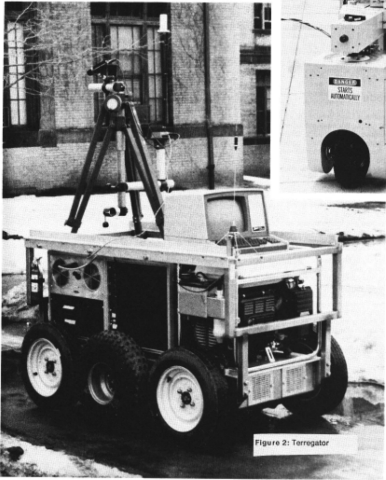
No mobile robot system is complete without a mobile robot. The primary vehicle of the CMU ALV project is the Terregator, built in the Civil Engineering Department. The design and construction of the Terregator (for lerrestrial navigalor) is docurnented in [7]. 1t is a 6-wheeled vehicle, 64 inches lang by 39" wide by 37" lall. All wheels are driven, with one motor for the 3 left wheels and one for the 3 right wheels. Shaft encoders count wheel turns, but the vehicle skid-steering introduces sorne indeterminacy.

The Terregator is untethered. Power is provided by an on-board generator. Communications with a hast computer are via a bi­ directional1200 baudradio link for vehicle status and commands, and a 10 megahertz microwave link for television signal from the vehicle to a digitizer. A remote VAX 11/780 runs programs for symbolic processing of visual data and navigation. A Grinnell GMR 270 attached to the Vax computes low- Ievel visual Operations such as edge detection. A Motorola 68000 on the Terregator translates steering commands from the VAX into wheel velocities for the left and right wheels.

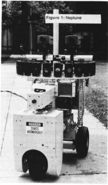
Earlier work also used the lethered robot Neptune, built by the Mobile Robot Lab. Neptune is a simple tricycle, with a powered and steered from wheel and two passive wheels in the rear. lts sensors consist of two cameras (for stereo vision work), ;>lus a ring of 24 sonars. While it was intended prirnarily for indoor work, it has !arge enough wheels to run outside on gentle terrain. With suitable modifications (an umbrella taped to the camera mast), it even has limited all-weather capability.

Our first successful continuous motion road following was achieved with Neptune running in our Iab on a road marked with black electrical tape on the floor. This 5 meter road had one left turn and one right turn, which Neptune navigated successfully. At the end of the road, Neptune made a sharp right turn and drove araund in circles.

The Vision and Navigation Program

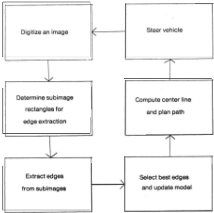
The primary task of our vision and navigation program is to keep the vehicle centered on the road as it rolls along at a constant speed. The program accomplishes this task by repeatedly digitizing road images, locating the road edges in the image, calculating the deviation from the center line, and steering to realign the vehicle.

The program was designed to be fast yet reliable. While the vehicle is moving along a planned path, an image is digitized.

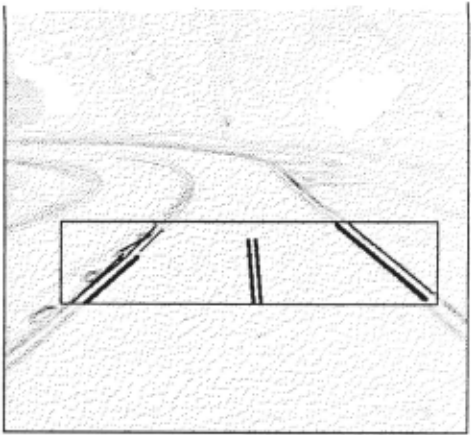
Since images are digitized frequently , the appearance of the road edges cloes not change appreciably across successive images; consequently, searching the entire irnage is unnecessary. ln order to constrain the search, the program maintains a model of the road The model contains the position and orientation of the left and right road edges seen in a recent image. The program uses these model edges to generate two small subimage rectangles in which to search for the left and right road edges. Since the approximate direction of each road edge is known a priori , the program uses directed curve tracing to reduce processing time and to preclude spurious edges. Generally the program finds more tilan one edge in each subimage rectangle. The model is used to select the pair of extracted edges most likely to be road edges. This new pair replaces the old pair in the model. From the model pair, the program computes a center line, the vehicle's dritt from the center line, and a steering command to bring the vehicle closer to the center line. As the vehicle executes a steering command another image is digitized and the cycle repeats. Figura 3 depicts the program control flow. ln the remainder of the paper we explain each component of the program in greater detail.

Constraining the Search

Each time the program digitizes an image it chooses two subimage rectangles to constrain the search for left and right edges. The representation of the reetangle is two horizontal and two vertical bounding line segments. The vehicle always "Iooks" a fixed <:iistarice ahead; therefore, the placement in the image of the horizontal bounding segments is predetermined and remains fixed across successive images. The placement of the segments is partly determined by two parameters selected manually: the height of the reetangle (typically 50 to 100 pixels) and reetangle overlap, that is, the percentage of the road in a reetangle seen in the preceding image (typically 50%). These two parameters present important Irade olfs: II a !arge height is chosen, the extracted road edges will be langer, thus providing more accurate information about the road; however, the processing time will be increased , and the road will be scrutinized less often. II a large overlap is chosen, more inlormation is available from the previous image and spurious edges are less likely to deceive the algorithm; however, the vehicle's speed must be siowed to enable such overlap. The two parameters, coupled with the vehicle's speed, the image processing time, and the camera's tilt determine the placement of the horizontal bounding segments in the image.

The vertical bounding segments change from image to image. The program selects bounding segments so that the road edges, based on predictions from the model and a preset error tolerance, will appear within the rectangle. This error tolerance arises from two sources: First, the program obtains its estimates of the vehicle's motion by dead reckoning, which is somewhat inaccurate. Second, the program assumes the road is straight, that is, predictions are made by linearly extending the road edges. Road curvature introduces a discrepancy between these predictions and the actual road; consequently, the ;·ectangle must be wide enough to see the road edge within a preset tolerance.

Selecting the Best Edges

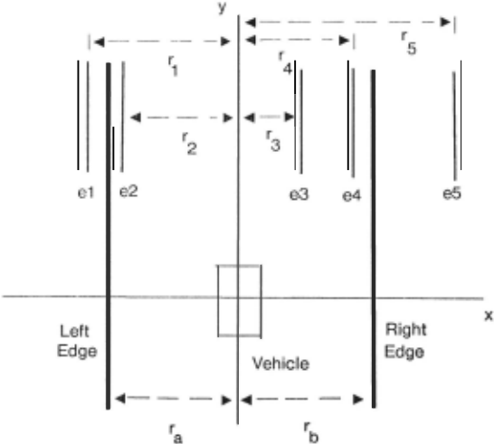
The line finding routine generally returns more than one line from each rectangle. The program passes these lines through a nurnber of filters to determine which, if any, are road edges. The new road edges are used to plan a path for the vehicle and to update the model. The 16 best left and right edge candidates (based on weights supplied by the line finding routine) are retained, and the rest are discarded. The program assu:nes that the camera's calibration, position, and orienlation with respect to the road are known , that the ground is locally Ievei and that all candidate edges arise from ground features. These assumptions allow the program to project each candidate edge into a unique hne 1n the ground plane. We establish a righthanded coord inate system with the vehicle at the origin and the xy-plane on the ground, with the positive x-axis directed to the right of the vehicle and the positive y-axis directed forward . For eacll transformed edge, the program calculates the following pararneters: the perpendicular distance r measured from the origin to the edge and the angle 0 measured from the positive x-axis. The differences in r and 0 between each transformed candidate edge and the corresponding model edge are calculated (call these values dr and dO respectively). The quantity dr is the difference in displacements of the vehicle from the model edge and from the candidate edge. The quantity dO is the angle between the rnodel edge and the candidate edge. Test runs have shown that the veh1cle tends to remain aligned with the center line; most of the error is in the form of lateral drill from this line. Hence, dr provieles the most information for evaluating candidate edges. The quantity dO tends to be small (less than 10 degrees); consequently, an early hlter uses it to eliminate spurious edges. After this round of edge elimination, one of three cases remains:

1. All edge candidatos have been eliminated
2. All edge candidates have been eliminated for a particular road edge (eitiler left or right)
3. At least one edge candidate remains for both the left and right road edge

ln the first case, the program obtains no new information and the vehicle continues to execute the path planned from the previous image. ln the second case, only one road edge is visible. The other road edge is occluded, shadowed, or poorly defined. Suppose for example the program found a set of candidate road edges an the right side but none an the left. From the candidate edges on the right side the program selects the one with the minimum dr value. lt inserts this new edge into the model, retains the old model edge for the left side, and generates a newsteering command. ln the third case, both road edges are visible. The program selects one edge from each Iist of road edges (lelt and right) by comparing each left edge to each right edge candidate and choosing the pair that minimizes the difference in their dr values, that is, it selects the two edge candidates that differ from ~heir corresponding model edge in the same way. Figura 3 1llustrates road edge selection in this case. This decision is based an the Observation that vehicle motion error and road curvature shift the location of each edge in the image in the same way. The program inserts the two new road edges into the model and plans a new path.

Line and edge cxtraction

At the lowest Ieveis of the vision system for our vehicle, the edge and lme extract1on modules. we found that for detecting road edges we could rely on the principle "almost anything works in the simple cases._" That is, any of a number of simple ~dge and line fmdmg techn1ques could be used to extract road edges in various Situations. Our approach then was to try everything. We tested various edge and line finding programs on static road images and on images acquired by the vehicle in actual runs. Simple techn1ques proved adequate in rnany situations we encountered.

The basic approach of all the vision moduies we tried was to find thc left and right boundaries of the road and represent them as lines. Therefore, the task of the low Ievei vision modules is to find line segments which are plausible candidate road edges. We sought to make only the most general assumptions about what might constitute a road in an image. The technique used to extract road t.'<lges and represent them as lines depends on whether we !hink of a road as an intensity change from background , a texture change, a color change or a combination. We experirnented with 7 metlwds for ex tracting road edges frorn irnages and three rnethods for fitting lines to the edges. The seven techniques we used to find edges in road images were:

1. Correlation. Assuming that a road edge is a more or less vertical feature in a subimage it can be followed by selecting a small sample patch of the edge and correlating this on a row-by- row basis with the subimage. Where the correlation is st;ongest in each row a road edge elernent is assumed. The result is a Iist of points where the road edge appears in each row. A line can be fit to these directly. The correlation approach worked very weil when the sample road edge patch was hand selected.
2. DOG operator. A Difference of Gaussian edge operator was tried at a wide range of spatial resolutions on road images. Road edges tend to be low spatial frequency signals so !arge DOGs were required to find them directly. Two-dimensional DOG filters tended to break up the road edges even at low frequencies. One dimensional DOG operators applied horizontally in the image produced more connected road edge pieces, since the road boundaries were almest vertical features in the image. High spatial frequency DOG operators can be used as the basis of a texture-based segmentation of road images, however.
3. Temporal Edge Detector. Subtracting two successive image frames is an inexpensive method for detecting image features that change from one moment to the next. II a vehicle is traveling down an ideal road (where the intensity of the road is uniform, the intensity of the surrounding region is uniform and the road edges are straight and parallel) then the difference of two successive road images is zero. When the vehicle begins to turn left or right oft the road, however, simple image differencing finds the road edges. This strategy was used in one experiment to servo Neptune visually down a hallway. Here the road edges were particularly distinct so the idealness assumption was more or less satisfied.
4. Roberts Operator. A 2x2 Roberts edge operator was sufficient to find road edges where they were relatively well -defined intensity step functions, such as when the vehicle lraveled down a hallway or when we artificially marked the road edges with tape.
5. lntensity Segmentation. A simple binary intensity segmentation of the road image works in many cases where the road is a set ·Of pixels most of whose intensities are grouped Iogether in the image histogram. We used a simple segmentation technique based on classifying all the pixels in the bottarn 50% of the histogram as one region and those in the upper 50% as another. Standard procedures for expanding and shrinking the resulting segments to join closely spaced segments and eliminate small ones are applied. Road edges are assumed to lie along the boundaries of the resulting regions.

1. Texture Segmentalion. Texture based segrnentation often proves better than intensity based segmentation for road edges where the road is relatively srnooth and the surrounding region is not, such as when the road is asphall against a grass background. A simple Iexiure operator which we have found useful in detecting road edges is one which counts lhe nurnber of edges per unit area and classifies all those areas where the edge count is high as a single region.
2. Row Integration . Summing the intensi ties column­ by-column in a set of scanlines in the image results in a single-scanline intensi ty image where the road is roughly a one dimensional box function. given that the road is a more or less vertical feature and the road and surrounding area each have fairly uniform but different intensities. Finding the boundaries of the box amounts to finding the average position of the left and right road edges over the scanlines summed. Repeating the procedure foranother set of rows in the image locates another pair of road edge points which can be joined with the first to approximate the road boundaries as line segments.

The three line-extraction techniques we used were:

1. Least Sqau res Line Fitting. When we had only one possible line in an edge image, such as the result of running a correlation operator over the rows or collecting a number of road edge points by row integration, a line could be fit to the points by least squares.
2. Muff Transform. A modified Hough (Muff) transform was used to fit lines to edge data where the edge extractor returned points that could plausibly be parts of several lines. The Hough transform has been used to detect road edges in other road findinq programs [6) [1]. The Muff transform uses a new parameterization for lines in images. 1 he Muff transform has several implementational advantages over the conventional p-8 parameterization. The details and implementation of the Muff transform are presented elsewhere [5].
3. Line Tracing. Most of the subimages we processed to find lines were bands about 50 pixels lall and 250 pixels wide. A simple rasier traclüng algorithm found in [3) proved sufficient to trace the road edges. Basically, if an edge point P above some high threshhold d is found while scanning the subimage, then we search on scan lines below for connected edge points above some lower threshhold t. The last such point found in the subimage is called Q and we assume PO is a line segment. The line tracing procedure is much like the inverse of a Bresenham algori thm for drawing lines, with the similar Iimitation that we can find lines that are only with 45 degrees of vertical. We find lines more than 45 degrees from perpendicular and lines with gaps by search ing in a neighborhood below an edge point for the next adjacent eclge point. Strictly speaking. our tracing program returns the endpoints of a curve which may not necessarily be a line, but over the ·small distances in the subimages we search for lines we have found this fast tracing procedure yields an adequate approximation. The line iracing procedure was used in all of the real time continuous motion runs of our vehtcle under vision control.

A combination of three factors enabled us to reduce the image processing time for each image sample to about 2 seconds. First, special image processing hardware in our Grinnell GlviR 270 display processor was used for the low-level correlation and convolution. Second , only small subimages (50 by 250 pixels) were searc l1ed for road edges by the line finding routines. Third, selection frorn among the possible set ot candidate road edges ot the actual road edges was accomplished by simple means (q.v.).

The next step in our plans for development of low-level road­ finding vision is to mtegrate several types of feature detectors in a blackboard cfata structure. We want to ev<J iuate the success of cornbini ng intensity, texture and c::o lor edge ancf region features to find road edges. Earlicr we said that we relied on the principle "almost anything worl1s in simple cases". For complicated cases, such as we have encountered i01 ac: tual outdoor road scen8s, we have tound !hat none of the techniques we have tried always works. We believe that a combination ot techniques will enable us to find road edges reliably in a wide range of situations.

Control

The control procedure translates the visual measurements into vehicle motor commands that , if successful , keep the vehicle moving along the road. We evaluated a half-dozen approaches experimentally with our vehicles and analy1ically. One approach, servoing to keep the road image centered in the torward field of view, excelled in all the measures, by such a margin that we teel it deserves to be considered a fundamental navigational pnnciple for mobile robots.

Let x represent the shortest distance between the center of our vehicle and the centerline of a straight road. 0 is the angle betwcen tlle heading of the robot and the road direction, i.e. when 0 = 0 the robot is driving parallel to the road . Suppose the vehicle travels at a constant scalar velocity v, and that control is achieved by superirnposing a steering rate, dO I dt (where t is time) on top of the torward motion. II there is no slippage, the following kinernatic relationship will hold:

The general problern for continuous road following is to find a steering function F such that by setting dO I dt = F(x,O) !he vehicle approaches th~ road center. We tried several functions and noticed a number of recurring problems. Estimating 0 and x from the image requires both a precise calibration of the camera and accurate determination of the position and orientation of the road edges in the image. 8oth are difficult to achieve in practice, and the high noise Ievei in these quantities made most of our functions unstable. A second problern led directly to our solution. The road image sometimes drifted out of the camera's 40 degree field of view, and in the next sampling period the program would fail to find a road , or (worse) identified some other feature, like a door edge, as road. The obvious solutionwas to servo to keep the road image centered. Experimentally this approach was a stunning success. Besides helping the vision , it seemed to be insensitive to even large calibration errors and misestimates of the road parameters.

The theoretical analysis was remarkably sweet also, and bore out the empirical observations. A first order analysis, where we assume the road image is kept perfectly centered, gives the relation

where r is the distance in front of the robot where a ray through the carnera image center intersects the ground (i.e. the range at which we do our road finding) . The parameter r can be changed by raising or lowering the camera, changing its tilt, or by using a different scanline as the center of the region in which road edges are sought.

Equation (2) can be substituted into (1) to give

which can be solved directly, giving

where x 0 is the initial value of x when t = 0, so to first order the vehicle approaches the centerline of the road exponentially with time.

A more detailed analysis considers the actual servo loop behavior. The displacement of the rcad centerline image from the center of the torward field of view is proportional to

Servoing the stcering rate on (5) sets

where g is the servo loop gain. The full behavior of the robot can be found by solving (1) with (6) simultaneously. These equations are made linear and easily solvable by the Substitution Q = sin 0, giving

By co-incidence or cosmic significance of all the servo functions we considered, only this one yielded a fully general analytic solution.

The solution has three cases distinguished by the sign of the expression

ln all cases the solution converges to x = 0, Q (and 0) = 0 exponentially with time. When g < 4v/r the convergence is a decaying oscillation - the sluggish steering causes repeated overshoots of the road center. When g > 4v/r the solution contains a secend exponential , and the robot approaches the road center more slowly. When g = 4v/r, the critically damped case, we have the fastest convergence and no overshoot, and the behavior is given by the equations

(9)

The gain sets the turn rate required of the robot. Note that to retain the critically damped situation while increasing v without changing g, it is necessary only to increase r, i.e. arrange to have the vision Iook further ahead.

The method is successful for several reasons. lt keeps the road in view at all Iimes. Because the system always converges, errors in g or camera calibration do not jeopardize performance. Because the parameter being servoed is the most robust direct measurable, namely road position in the image, the noise problems of the other approaches are almost totally eliminated. ln particular, 0 (or 0) and x though they occupy a central position in the theoretical analysis, need never be calculated in the actual servo loop.

Conclusions

We have developed a vision and control system for a mobile robot capable of driving the vehicle down a road in continuous motion. The system has been tested on two mobile robots, Neptune and the Terregator, in both indoor (hallway and artificial road) and outdoor (asphalt paths in a park and cement sidewalk) environments. ln our best run to date the Te1·regator traversed a 20 meter outdoor path at 2 ern / sec. Image processing time has been reduced to 2 sec/image.

Failure modes of our vehicle have included driving oll the road, driving into trees and walls, and driving areund in circles. Such failures were mostly due to bugs in our programs. imprecise calibration procedures. and limitations of current hardware (e.g., B&W camera with narrow angle lens). not fundamentallimitations of the techniques used.

Future Work

There are several areas that we plan to address. First is the construction of a true testbed. This involves mostly software engineering , such as cleaning up and documenting the interfaces between vision and control. This will enable us to try other vision methods, such as texture and color operators.

Further work will require the use of a map, along with program access to a magnetic compass and a gyro. The map will Iist road direction , width, appearance, and intersections, which will provide strong cues to both the image processing and the navigation system. The compass, along with the map information, will help predict road location in the image. This will become increasingly important as we venture onto curved and hflly roads, and as we encounter intersections and changes in the road surface.

The next step is obstacle avoidance, wtiich will require limited 30- processing . Projects in the CMU Mobile Robot Labaratory have already demonstrated obstacle avoidance with sonar [2] and stereo cameras [4]; we intend to integrale these into the testbed. Later work may add a Iaser rangetinder and programs to handle that data.

Finally, as the testbed becomes more complicated, system control will become a major issue. We plan to work on a blackboard system with cooperating and competing knowledge sources. All the data, from the lowest Ievei signals to the highest Ievei models and maps, will be on the blackboard and available to all processes.

Acknowledgements

We would like to thank first of all Pat Muir for his work on analysis of the control of the Terregator. Many thanks also to Mika Blackwell , microprocessor hacker extrodinaire, Kevin Dowling, tender of robots, and John Bares, prime mover of the Terregator, without whom the experiments described here would have been much more difficult and much less fun. Thanks also to Gregg Podnar and Bob Spies for video and digitization work. Finally, we would like to express our appreciation to Raj Reddy for his support and encouragement.