A Subdivision Algorithm Configuration Space for Findpath With Rotation

A SUUDlVlSION ALGOIUTllM IN CONFIGUHATION SPAC~ FOR FINDPATII WITIIIWTATION

Rodney A. Brooks and Tomas Lozano- Perez

MIT Artificial Intelligence L11boratory 545 Technology Square

Cambridge, Massachusetss, 02139, U.S.A.

the presc!ICC of the irnmovahif' obs!.acles some of'p;ions of the configur~tion space arc not re:1.chablc; these rc~;io n s are the configuration obstacles. llcnce, in t.hc configur<:lion space, the moving object is shrtJnk to a configuration point while the immovable obstacles arc expanded to fill all space where the presence of the configumtion point would imply a collision of the object with oostac!es. The findpath proble1n of finding a path for the object. through the original space while avoiding obstacles is thus tmnsformcd to linding a path for the confi1~uration point through the configuration space while avoiding the configuration obstacles.

The fundamcnt:1.l structure of the algorithm is extremely simple. Configuration space is first divided into rect:1.ngloids with edges parallel to the axes of the space. Each rectangloid is labeled as {1) empty il" the interior of the r~cl.angl0id nowhere intersects a configuration obsLack, {2) full if the interior of the rf'.ctang;Joid everywhere intersects the configuration obstacles or {3) mixed if thne are interior points both inside :1.nd outside of configuration obst:1.clcs. A free path is fou iHl by fir st fiJ!ding a connected set of empty rectan~lo;d cells t haL include the initial and goal configtJrations and constructing a piecewise li near path th rough those empty cells. If such an empty cell path cannot be found in the inilial wbdivision of configur.J.tion space then a path that includes mixed cells is fou11d. Mixed cells on the path arc suodi vided , by cutting them wit h a single planl' normal to a coordi nate axis, and each resulting cell is appropriately labeled as empty, full, or mixed. Anothe r sea rch for an cmpiy- cell p:1.th is initiated, and so on iteratively until success is achieved. If at any time no path can be found through non--full cells of greater than some preset minimum size, then the proulcm as posed is insoluble (i.e. , no collision free path exists given the resolution limit) .

The conceptual and practical problems that must be solved to implement this algorithm are as follows:

• (a) What is an eflicicnt algorithm for labeling the newly cut cells as empty, full or mixer!?
• (b) How should configuration sp:1.ce be initially divided into rectangloids?
• {c) vVhcre should a mixer! cell be cut when it is subdivided?
• {d) What. additional information should be krpt with mixed cells desc ribing the configuration space obstacles they intersect?
• (c) llow should the iterative sea rch be controlled?

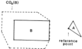
II. Representation of Confi~ul'ation Space Obstacles For a co~;~~ -p-;;-lyg~nal J~ov!~tg-~bj;;-Z~\-and a coJ;-;~-;-polygonal obstacle B we write the confl gurations forbidden for A as CO A{D). Figure 1 shows such a coioligur:1.tion obstacle for polygons A and D where their relati ve orientation is fixed. Lozano P erez [1983a] showed th:1.t COr~{ H), for fixed relative orientations of convex A and B, is also a convex polygon. A

ABSTRACT

A recursive cellular representation for configuration space is prcspnted, along with an :1.lgorithm for searching that space for co lli sion -free paths. The details of the :1.lgorithm arc presented for polygonal obstacles and a moving object with two transla­ tional and one rotational degrees of freedom.

I. Intr9_dJ!~ion

[n this paper we present an algorithm for finding collision- free path s for a rigid polyg;onal object moving through space that is cluttered with obstacle polygons. The paths can include rntations of the object. The algorithm will find a path from a given initial position and orientation to a goal position and orientation if such a path exists, subject only to a user- specified resolution limit on ciisplacements.

The problem addressed here is an instance of the problem known as the flndpatii or mover's problem in robotics. The problem arises when planning the motion of a robot manipulator or mobile robot in an environment with kno"vvn obstacles. For rei:1.Lcd app ro:1.ches to the findpath problem, sec Drooks [198~], Lozano-Perez [1981, 1983a], Lozano-Perez and Wesley [1979], tvloravcc [1080], Schwartz and Sharir [1981, 1982], and Udupa [1977]. A survey of the different approaches to findpath and a discussion of its role in robot task planning can be found in Lozano-Perez [1983b].

The algorithm described here is based on the configuration space approach described by Lozano-Perez [1981, 1983a.]. The configuration of a rigid object is a set of independent pammetcrs that characterize the posi Lion of every point in the object. We associate a local coordinate frame with a rigid object, such as a planar polygon. The configuration of the polygon can be specified by the x, y position of the origin of the local coor­ dinate frame, known as the reference point and a 0 value in­ dicating the rotation of the local frame relative to the global frame. The space of all possible configurations of an object is its configuration space. A point in the configuration space, a configuration point, r~presents a particular position of the ob­ ject's reference point and an orientation of the object's axes.

The configuration space for planar polygons is three­ dimensional while that of solid polyhedr:1. is six-dimen~ional: th ree trauslational and three rotational dimensions. Due to

This report describes research done at the Artificial lntellig('nce Laboratory of the Massachusetts Institute of Technology. Support for the Laboratory's Artificial Intelligence resea rch is provided in p:1.rt by t.hc Office of Naval Research under Office of Naval He~carch contract N00011- 81- K- 0191 and in part by the Advanced Research Projects Agency under Office of Naval fl.esearch contracts NU0011- 80 -C- 0505 and N00014- 82K- 0331.

' ' \--- ---------·

type B

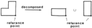
Figure 3. Non-convex moving objects can be decomposed into a union of convex objects sharing a common reference point and reference orientation.

convex polygon can be expressed as a conjunction of linear in­ equalities.

When changes in the orientation of the moving object are allowed, the resultant CO~(B) arc neither convex nor bounded by half-spaces. Their surfaceR are curved, although they do have the property that when cut by a plane normal to the rotation dimension they have polygonal cross sections (since such a cross section corresponds to a single fixed orientation).

Lozano--Perez [1983a) showed that for two dimensional A and B the surfaces of the configuration obstacle could be ex­ pressed as inequalities each valid over an infinite rectangloid R in (x, y, II) space, where

for some fixed lit and ll2 . These inequalities are of the form f(x, y, II) ~ 0 where f can be defined by either

or

where the ranges of validity are given by

and

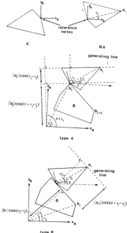
The a;'s are vertices of the "negated" moving polygon (8A in Lozano-Perez [HI81, 1983a]), in its local coordinate system. 1/. is the angle the line from the origin of that coordinate system to the point a; makes with the coordin11te system's x axis, and ),, is the angle made by the normal to the segment from a; to a;+ t· Similarly the b/s are the vertices of a convex obstacle polygon, 'YJ the orientation of the line from the origin to bi, and ¢ 1 the orientation of the normal to the segment from bi to bi+ t· The parameter 0, a parameter of the configuration space, measures the angle between the x- axes of the object and obstacle coordinate systems. Figure 2 shows the geometric con­ structions used to derive the forms of type A and B constraints.

Type A constraints can be thought of as being generated by a face (edge) of the moving object A coming into contact with a vertex of an obstacle B, and a type B constraint as a vertex of A coming into contact with a face (edge) of B.

We can cut up configuration space into rectangloids R;. For a sir.gle convex obstacle and a convex moving object (either with or without rotation) we can define the subset of the configuration space obstacle that intersects R, by those points in R; such that a conjunction /\, e; is satisfied, where each e; is an inequality.

In the more general case the moving object A is represented as a union of (possibly overlapping) convex polygons. Similarly, multiple obstacles are each represented as unions of convex polygons. Let the convex moving polygons be At,A2, ... ,An. Define a single reference point P and reference orientation for all the A;. See Figure 3 for an example. Let the convex obstacle polygons be Bt, B2, . .. , Bm.

The path for object A can be found through the obstacle lit­ tered space by finding a path for the configuration point through configuration space filled with the union of the CO A, (B1)'s or CO~. (Bi)'s. Hence, for arbi trary obstacle and moving object polygons, we first decompose t hem into the unions of convex polygons; lchen, for all pairs of obstacle and obj ect polygons we compute the configuration space obstacles. These new obstacles are all embedded in the same configuration space, and a colli sion--free path is found through it for the reference point of the object to be moved.

In what follows we will represenet an obstacle embedded in configuration space as a union of finite rectangloid boxes each 'vith edges parallel to the coordinate axes. The boxes will each have associated with them a conjunction of inequalities which will allow us to determine the subset cf the configuration space obstacle that intersects that box. We then embed these boxes into configuration space by cutting it into rectangloids.

The way in which the set of boxes bounding a particular configuration space obstacle is chosen is discussed in section IIB.

A. Representation of Configuration Space

The inequalities derived above are referred to as constraints. Each one has the form f(x) ::;; 0, where x is the configuration point for the moving object. A point xis inside such a constraint if f(x) < 0, outside if f(x) > 0 and on the constraint if f(x) = 0. A point is contained in a configuration obstacle if it is not ou tside any of its defining constraints. A point xis on the surface of an obstacle if it is on some constraint.

If two obstacles arc embedded in the same space and two of their bounding boxes interser.t then the two can be decomposed into a union of boxes. Each resulting box has associated with it a disjunction of the conjunctions representing the original two obstacles. Of course, the sub- boxes that only overlapped a si ngle configuration space obstacle have just the original con­ juncti on.

More formally, we represent configuration obstacles as fol­ lows. ConHguration space is subdivided into rectangloid cells in order to represent the embedding of many configuration obstacles. Each cell is a closed rectangloid with edges parallel to the coordinate axes. The u·nion of all cells is the whole space and no point is in the interior of two cells. Associated with each cell is a sentence of constraints of the form

Each conjunction of constraints in a sentence will be referred to as a clause and each clause is made up of terms, i.e., each constraint will be referred to as a term.

A point is said to be inside sentence S if for some clause of the disjunction it is not outside any of the constraints. A point is said to be outside sentence S if it is outside some constraint in every clause. A cell C with associated sentence S is labeled

as

1. empty if no point of C is insideS,
2. full if no point of C is outside S,
3. mixed otherwise.

The labeling is done as a by- product of trying to simplify sen­ tence S; see below.

B. Simplification of Constraint Sentences

Both while constructing the original representation of configuration space and when subdividing cells during search it is necessary to associate a constraint sentence S with a cell C. It may be the case that the cell is completely outside or com­ pletely inside some constraints in S . The procedure below both si rnplifi e3 S by removing such constraints and, as a by--product, labels the cell empty, full, or mixed.

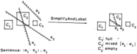
procedure SimplifyAndLabel (C, S); begin foreach CLAUSE in S do begin foreach TERM in CLAUSE do begin case CellCompare (C, TERM) of Inside: remove "fERM from CLAUSE; Outside: begin Cut: ; endcase; end; remove CLAUSE from S; goto next CLAUSE; end; if CLAUSE is nil then begin end; i! S is nil label C with fuJI set S to nil; exit from SimplifyAndLabel; end; then label C with empty else label C with mixed; end;

A sub-procedure Ce!lCompare is used to compare a cell C with a single constraint, e say. It returns one of:

1. Out,side if no point of Cis inside e,
2. Inside if no point of C is outside e,
3. Cut otherwise.

The formulation of CellCompare depends on the form of c.onstraints to be considered. Note also that in general the surface of a constraint (i .e., those points on the constraint) is of lower dimension than the configuration space in which it is embedded. Thus a constraint fills only a subset of measure zero of a cell.

C. Comparing a Cell to a Single Constraint

The idea of treating the spatial and rotational components of con figuration space uniformly breaks down when comparing a cell to a constraint. This is because the constraint surfaces are, in some sense, "well behaved" with respect to x and y, but "poorly behaved" with respect to () - the surfaces can creep into, and out of a cell along an edge in the() direction, while the vertices at both ends are on the same side of the constraint.

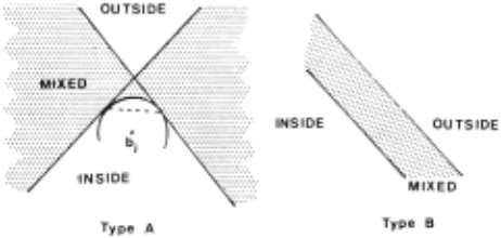
For a fixed Oo both type A and type B constraint surfaces become a single, infinite, straight line. Type A and B con­ straints are, therefore, ruled surfaces, which are valid over some range [Ot, 82]- Consider the projec.tions into the x- y plane of the portions of these surfaces in the range [01, 02] (slice projec­ tions in the terminology of Lozano-Perez [1981, 1983aJl. Points outside the projection must support columns in the () direction that are either completely inside or completely outside the con­ straint. Furthermore, there will he two disjoint regions outside the projection that correspond to these types of columns. Figure 5 illustrates the projection of both a type A and a type B con­ straint.

Thus the procedure CellCompare has been reduced to two more primitive operations; projection of the constraint surface into the x- y plane, and comparison of a rectangle to the two regions of the plane outside of that projection. If those regions are convex then the comparison is simple, as a convex polygon is contained in a convex set if and only if all its vertices are contained in the region.

A type B constraint projects into a strip with parallel sides. On one side is a half plane corresponding to points inside the constraint, and on the other a half plane corresponding to points on the outside. The comparison computation it trivial.

Type A constraints are considerably more difficult to deal with, as t~e orientation of the ruled line on the constraint surface rotates with changing 0. Consider Figure 5. Note that again both the inside and outside regions are convex, so a projected cell vertex test suffices. A point is in the outside region if it is outside both of the straight lines. It is inside if it is inside both of the straight lines and not in the small area between the circle and the point of intersection of the two lines. Such points have distance from bi greater than the radius of the circle, and are on the opposite side of the chord (joining the two intersections of the circle with the straight lines) as point bi.

Full details can be found in a longer version of this paper: [1982].

D. Bounding Configuration Obstacles

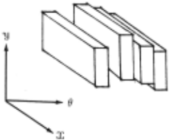
In this section we describe how the set of bounding cells for each configuration obstacle is chosen. As 0 varies, the x and y bounds on the 'cross section of CO~(B) normal to the 0 axis varies considerably. Hence it is best to bound CO~(B) by a "stac.k" of cells in the 0 direction; see Figure G. The cells are obtained by, first, determining a number of sub- intervals of the complete 0 range and, second, determining the x and y bounds of the configuration obstacles over each sub- interval.

The sub- intervals are chosen as follows. The interval [·-7f, 1r] is cut at all values of the form 2n7f + Ai -- ¢J that, for some integer n, lie within the interval. Any constraint that is valid for some interior point of one of the resulting sub- iatervals is taken as valid over the whole closed sub- interval.

A conjunction of all valid constraints over a sub- interval forms the initial constraint sentence of a cell whose 0 range cor­ responds to the sub- interval. Later the cells will be embedded in the configuration space, and will perhaps be intersected with other cells, whence their constraint sentences will become dis­ junctive terms of new constraint sentences.

For a cell whose 0 interval is [01, 02], the maximal x value, achieved over the points that satisfy its constraint sentence, must occur at a point that has a 0 component within that interval. Let the () component of this maximal point be Oo. By convexity, the maximal point must be a vertex of the convex polygon that is the cross section of CO~(B) at 00 · For a fixed 00 , Lozano- Perez [198.3a] showed that this cross section is the convex hull of all points of the form

where ai = (a,., aiy) and b 1 = (b 1 ., bJy) are vertices of A and B, respectively. The maximal x value must be achieved at one of these points, which can be identilled by maximizing the expressions above over values of 00 in the legal range. Similar computations determine the minimal value of x and the extreme values of y.

E. Constructing an Initial Representation

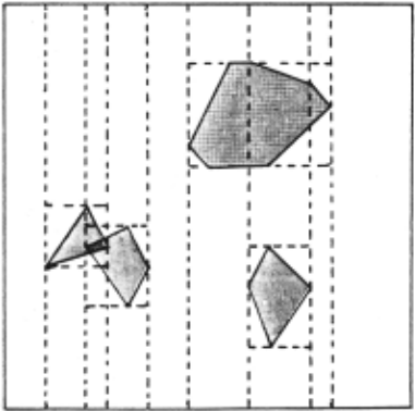
We arc now in a position to construct an initial representation of configuration space. There are two operations. (1) Cut space into rectangloid cells. (2) Build a connectivity graph between the cells which are empty or mixed. By combining the second operation with the first it is possible to reduce its complexity to linear in the final number of cells. Full details can be found in a longer version of this paper: [1982]. The computation (as distinct from the actual algortihm) uses all the extreme x, say, values of bounding boxes to cut configuration space into strips and intersects all the boxes with those strips, cutting them when necessary. Then each strip is cut with all the extreme y values of boxes which lie within that strip. The process is repeated for each axis of configuration space.

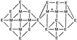
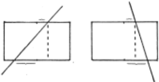
Figure 7 shows a configuration space for polygons without rotation cut into rectangular cells. A cell is represented by a rec­ tangloid, a constraint sentence in constraints that cut it, a label from among full, empty, and mixed, and pointers to neighboring cells. The neighbors are grouped according to their direction, e.g. +x, -x, +y, and -y for two dimensional configuration space. Figure 8 shows its corresponding connectivity graph.

An important refinement to the simple connectivity graph is possible. Two neighboring cells C1 and C2 intersect in a rectangloid cell C one dimension lower than the original cells. Both constraint sentences St, from Ct, and S2, from C2, apply to the intersection cell. If either SimplifyAndLabel(C, St) or SimplifyAndLabel( C, S2) label C as full then the configuration point cannot move directly from cell C1 to C2. Hence, although spatially neighbors, none of their empty interior points are con­ nected by a path for the moving object's configuration point. Thus their neighbor relation can be omitted from the connec­ tivity graph. For this reason, link A of Figure 8 can be deleted.

This refinement significantly cuts down the number of links in realistic connectivity graphs, greatly inc.reasing efficiency.

A major drawback to cellular representations as above is that a r.umber of small obstacles localized in one part of space can have significant global c!Tects on the representation of space elsewhere, e.g., the effect of x bounds in Figure 7. This can become a signillcant problem in three--dimensional configuration space.

This problem is solved by first boxing the stack of 8 slices for a single configuration obstacle into a single cell that extends over the range [-1r, 1r] in the 0 direction. Such cells are em­ bedded into the configuration space that is sliced in the x and y directions. Then, within each cell, the cutting procedure is used all over again, first cutting normal to the 8- axis then normal to each of x and y.

The efficiency of the algorithm can be further enhanced by arranging for the second stage of cutting to be carried out only when it first becomes a candidate path cell as found by the A' search algorithm.

m. fu!arcili_

The representation described above for configuration space is useful only if some efficient way can be found to search it for collision- free paths. Our algorithm uses the A' (Nilsson [1971]) algorithm as its primary search engine to search the cell con­ nectivity graph, bot.h for paths through purely empty cells and for paths that include mixed cells.

Once a set of empty cells linking the initial point to the goal has been found, an actual point path through those cells must be chosen. Again the A· search procedure is used, but this time using a selected set of points in the cells along the solution path.

If no path through empty cells is available, then the rep­ resentation of configuration space must be refined through cell division. It is necessary, however, to decide where the space should be refined, and how much effort should he expended in subdivision, before a new search is initiated. The point path search mentioned above is used to direct the refinement of configuration space as well as to produce a final solution path for the problem.

The efficiency of the overall search can be greatly improved by using the divide and conquer paradigm. There are some complications in this application, however, as each subproblem is capable of changing the global data base by refining the representation of space within its area of search. This turns out to be a significant problem and some care must be taken to minimize its adverse e!Tects. There is an additional problem with divide and conquer in this application. The division of a problem into subproblems cannot guarantee that if the original problem is solvable then so are all the subproblems. A form of resource limited computation is used to back out of problem subdivisions that do not look promising.

A. Deciding Where to Cut a Cell

During search, the representations of mixed cells that lie on the candidate path are refined. A cell C with sentence S is cut into two cells, C1 and C2 , by splitting along one of its coordinates. Then, each sub-cell is labeled by calling SimplifyAndLabel( C;, S) fori = 1, 2.

The cutting operation can help the search converge on a. path through empty cells but only if it makes it easier to deduce if at least one of the C;'s is full or empty. This will be the case if the number of constraints appearing in at least one sen­ tence S, is reduced from the number that appeared in S. Such simplification can be achieved if one of the new cells lies wholly inside or outside a constraint. We refer to it as the simpler sub-cell.

Two heuristic principles have also been used in the imple­ mented algorithms described here. First, it is desirable that the new cell with simpler constraint sentence should have the max­ imal volume possible. This offers the possibility of finding that a large volume is either empty or full. In one case it makes the search for a free path easier and in the other eliminates a large volume from further consideration. The second heuristic prin­ ciple is that large amounts of computation in choosing the place to cut a cell, would be better spent in cutting the cell into more, less well chosen, pieces, as more r:uts result in greater likelihood of actually finding empty or full sub- cells.

Thus there are three problems; (1) find cuts that lead to simpler S1 and S2; (2) choose the one that gives the simpler cell a large volume; (3) compute (1) and (2) quickly. Here we show how to choose a good cut according to these criteria. The method is stated in more generality than necessary so that it can easily be extended to the higher dimensional cases later in the paper.

The basic approach is as follows. Consideration is given to cutting the cell in each direction (x, y and 0 in this case) at some number of points for each constraint in the cell's constraint sentence. Candidate cuts are chosen wherever a constraint sur­ face will go through a vertex of one of the new cells. A score is assigned to each such plausible cut, and the cut with minimal score is chosen as best.

It remains now to define the scoring function. If the length of the cell in the x direction is scaled to 1.0 then the score of a cut is its distance in those units from the center in the x direction. Note that this score is a proportion of the volume of the original cell that is added or subtracted from half its volume to get the volumes of the two new cells. Thus the scale of this measure is independent of the constraint or the direction of cut. The same scoring function is used in the y and 0 directions.

If a given constraint and direction of cut produces two candidate cuts then in configuration space without rotations the one with lowest score is the one that produces a simpler cell with maximal volume (helping in the achievement of (2)). This can be shown by considering two cases, illustrated in Figure 9. It does this without analysis of the constraint other than where it cuts the edges of the cell.

In our implementation we choose the cut by picking the candidate with the lowest score from among all cutting direc­ tions and single constraints. This has the effect of choosing a cut that produces a simpler cell with volume closest to half the original cell volume. The chosen cell may not be the best pos­ sible choice in terms of condition (2), but it is certainly not a poor choice. If all possible simpler cells have volume less than haff the original, then this algorithm will in fact choose the cut that results in the largest such cell. If there are cells bigger than half, then the biggest one might not be chosen; condition (3) is well satisfied, however.

B. A · Cost Functions

While searching for a path of connected cells, a candidate point path through each partial cell path is "constructed". Each adjacent pair of cells intersect in a cell of one lower dimension. In the case of two dimensions without rotations, the interaction cell is a line segment and the centroid its midpoint, for example. The centroids of such interaction sub- cells are used as the entry and exit points of the path through the cell, and a the path segment within a cell is the straight line joining them.

The cost of an individual path segment is just its Euclidean length within the configuration space, and the cost of a path is the sum of the segment costs. The lower bound heuristic estimate for reaching the goal point, is just the Euclidean length from the last point on the path to the goal point.

The running time of the search algorithm can be improved by making the cost of traversing a mixed cell greater than the cost of traversing an empty cell. The relative cost can be used to trade off running time of the search algorithm for length of the final path. With a large relative cost, the A* algorithm will strongly tend to concentrate on empty cells. Hence, paths that require only a small amount of additional trail blazing through mixed cells will be chosen, even if they are very long.

C. Choosing a Point Path

When a final cell path consisting of empty cells has been found it is still necessary to find a path for the configuration point of the moving object through ·configuration space. In general, the choice of final path should be based on domain-specific considerations such as kinematic or dynamic characteristics, not on purely geometric criteria. In the absence of domain­ specific considerations we suggest that a desirable property of the final path is that it be smooth, essentially nulling out the artificial effects of the tesselation of configuration space by the cell structure. Our approach is to consider alternative paths going through a small set of candidate points in the interaction cell between adjacent cells in the chosen path, and to choose the one that minimizes the cost function by another A · search with the same cost function as detailed above.

D. Refining the Search Spac~

After a search has found a sequence of empty and mixed cells, the mixed cells along the path should be cut into at least two sub- cells and the search re- executed. This simple strategy leads to a very slowly converging search algorithm, however. The ratio of cutting to searching is too low. Arbitrarily cutting cells can also be wasted effort, however, so it is better to find some selective method of determining places to make more cuts. We use the point path search to identify such places.

The point path search of the previous section is used to find a point path through the empty and mixed cells. All points at the interface between cells on that path are then examined. It is easy to determine if a point is actually in free space by evaluating the constraint sentence associated with one of the containing cells. If the point is actually in free space, but its cell is mixed, then the cell is repeatedly divided until the point lies in a newly created empty cell. (This same procedure is used to cut the space representation about the initial and goal points to get empty initial and goal cells for the original search.) The effect of this is to create small islands of empty cells along the trajectory, which will be useful for defining recursive subproblems (see next section).

Initially there may be many large cells in the configuration space representation. If an arbitrary point on the interface between two adjacent cells were chosen as a center of refinement of the cell representation, it could well be that it is far from the optimal path. By only expanding points on a candidate optimal path, the overall search operation is not misled into grossly suboptimal areas of "easy pickings".

E. Divide ~~~_«!Conq':l_e.!:

The efficiency of the search for a free cell path can be greatly improved by hierarchically decomposing it into more localized and smaller problems. The search space is smaller for a localized problem, resulting in reduced time for the overall search.

The problem is how to break up a global search into smaller ones when there is no a priori knowledge of what the smaller subproblems are. The approach taken here is to use the global search through mixed cells, and subsequent selection of a point path as a plan for the lower level subproblems. If there are points on the path that, after cell refinement as above, are in a known empty cell, then they are used as points at which the problem is broken up. The global problem then becomes a series of local ones, each from an initial point to a goal point where both are in empty celts.

Surprisingly, the order in which the subproblems are at­ tempted is important. This is because each subproblem may require that the global data base, the cell connectivity graph, be altered, as mixed cells are cut. If the subproblems arc evaluated with the one closest to the global initial point first, and followed sequentially by those closer and closer to the goal point, then this cutting -has adverse effects on search efficiency.

Consider the first subproblem in a sequence. In general, many cells near the goal point will have been refined by the time a sub- path through empty cells has been found. Now the second subproblem is attacked. Its initial point is the goal point of the previous subproblem. When the A · search starts at that point it finds many small empty cells from the recent search. These cells arc in the wrong direction relative to the new goal, however; they are, nevertheless, "attractive" to the search algorithm, because the evaluation function favors empty cells. In addition the empty cells are small and, therefore, many can be appended to partial paths near the new initial point without sharp increases in the heuristic estimate of remaining cost. The result is that the A* algorithm can spend inordinate amounts of time breadth--first searching backwards over areas covered by the previous subproblem.

Fortunately, this wasted work can be avoided by solving the subproblems in the reverse order - taking the one nearest to the global goal point first.

Another consideration in the use of divide and conquer is the possibility that a subproblem may be poorly chosen so that there is no very direct path between its initial and goal points. This can be the case even when the global problem is soluble. If unlimited effort is expended on solving the subproblem then it can· happen that the final path "backs" out from the initial point, finds a· path around the obstacles that block a more direct route from the initial to final position, then "backs" into the goal position. The two subproblems on either side backtrack over those initial and final parts of the path. See Figure 10 for an illustration of this effect.

In such cases, after some effort has been expended to deter­ mine that the direct path is blocked, it is better to back up to the more global problem and look for a new path through mixed cells. This can be simply achieved by placing a path length limitation on sub-problems. Once it is exceeded the subproblem exits with failure, forcing a new search at a higher level. In the examples given in this paper the cost limitation for subproblems is 1.5 times the cost of the global path, or 1.5 times the best cost ever computed for the sub-path, whichever is smaller.

IV. Conclusion

The algorithm described here has been implemented and tested on many randomly generated examples. Figure 11 shows two difficult cases that the algorithm solves. We believe these to be among the most difficult find path problems ever solved by a pro­ gram. The running time of the algorithm on these examples is very high, however. The actual running times for these difllcult problems are on the order of tens of minutes of "wall- clock" time on a single- user MIT Lisp Machine without floating point hardware; these times also include a very significant paging over­ head. Simple problems, of course, run much faster: on the order of tens of seconds to a few minutes. This should be contrasted with running times on the order of less than a minute for prob­ lems of moderate complexity using the algorithm described in Brooks [1982]. This latter algorithm cannot solve problems such as illustrated in Figure 11, however.

While the running times of the algorithm described here could be made significantly shorter by implementation changes, the fact remains that the complexity of the algorithm is high. Informal timing experiments seem to indicate that the algorithm spends much of the running time in the A' search procedure, which is used at several points in the algorithm. If the number of cells to be searched could be reduced, the running time could be significantly reduced. One approach to doing this is to use an algorithm such as described by Brooks [1982] to identify a likely path, using a smaller and simpler moving object, and then apply the algorithm described here to verify and refine the path for the actual moving object. This would reduce the size of the search space for the algorithm. There arc a number of conceptual and technical problems to be solved before this hybrid approach is practical. As of now, the algorithm described here can solve very complex problems, albeit slowly.

The questions (a) through (e) posed in section 1 have been answered for the case of polygons with rotations. Section IlA addressed question (d), liB and liC addressed (a), liD and liE addressed (b), IliA addressed (c), and llHl, IIIC, IUD and IIIE addressed (e). In generalizations of the solved problem case it is necessary to further refine only a subset of these andsers.

The approach followed in this algorithm can be directly applied to configuration spaces for three-dimensional polyhedra whose orientation is fixed. This case generates a three­ dimensional configuration space with linear constraints - all of section 2 applies in simplified form. We believe that the generalization to a four-dimensional configuration space, such as for a polyhedra with a single rotational degree of freedom, will be straightforward . A new type of constraint surface must be dealt with, however, arising from the interaction of pairs of edges (Lozano-Perez [1983a]) .

The approach could, in principle, also be generalized to configuration spaces of higher dimension, such as those for polyhedra that are allowed to rotate. The actual generaliza­ tion presents a large number of problems, e.g., the CellCompare operation is substantially more difficult, and the number of cells grows extremely fast. Other algorithms suggested for this general case have the same drawback. The algorithm for the general findpath problem given by Schwartz and Sharir [1982], for example, has a very high polynomial time complexity for a fixed number of degrees of freedom and is exponential in the degrees of freedom. Our belief is that, in practice, the general six degree of freedom problem should be heuristically reduced to cases involving four or fewer degrees of freedom.

ACKNOWLEDGEMENTS

The presentation of this paper has benefitted greatly from the detailed comments of John Hollerbach and the IJCAI referees.