
Description of Textures by a Structural Analysis
Proceedings of the Sixth International Joint Conference on Artificial Intelligence. .
© 1979 International Joint Conferences on Artificial Intelligence
Abstract
We introduce a method of a structural analysis for description of textures in natural scenes. The proposed texture analysis system automatically extracts the elements in a texture image , measures their picture properties, classifies them into some discriminable classes (one "gr o und" and some "figures"), and produces the description of elements in each class and also of their placement rules. This description can be used for learning and recognition of texture images. We also present a new idea for evaluating texture analyzers. In order to directly see what essential features or structurs of the given textures each analyzer extracts, we propose an analysis-by-synthesis method. That is, the synthesis program in our system reconstructs the texture image on the basis of its description. Comparing the reconstructed image with the original one, we can evaluate what information is preserved and what is lost in the description and c an improve our algorithms.
- Lipkin, B.C. and Rosenfeld A. (Eds,): Picture Processing and Psychopictorics, Academic Press (1970),
- Tomita, F., Yachida, M, and Tsuji, S.: "Detection of homogeneous regions by structural analysis," Proc, 3rd Int. Joint Conf. on Artificial Intelligence, p,564 (1973). IJCAI
- Tomita, F., Shirai, Y., and "Classification of textures by a analysis," Proc, 4th Int. Joint Pattern Recognition, p.556 (1978), Tsuji, S.: structural Conf. on
- Weszka, J.S., Dyer, C.R., and Rosenfeld, A: "A comparative study of texture measures for terrain classification," IEEE Trans. SMC-6, p.269 (1976).
- Rosenfeld, A. and Kak, A.C.: Digital Picture Processing, New York: Academic (1976).
- Pavlidis, T.: "A review of algorithms for shape analysis," Computer Graphics and Image Processing, 7, p.243 (1978).
- Brodatz, P.: Textures, New York: (1966). Dover
- Marr, D.: "Early processing of visual information," MIT AI Memo, No. 340 (1975).
References were extracted automatically from the PDF and may contain errors.
Full text extracted automatically from the PDF; figures, tables and equations may differ. The PDF is the version of record.
1. INTRODUCTION
When we observe objects in a scene, we use the
textural information as follows.
- identification of objects by the categories of textures,
- discrimination of differences of textures, and objects by the
- perception of a depth, a or a inclination of a surface textures. curved surface, by the changes of
Endowing machines with these recognition capabilities is not only an interesting problem in computer science but also practically important for automatic analysis of aerial photographs or medical images. Texture has been studied on at least two levels: statistical and structural [1]. On the statistical level, we regard a texture as defined by a set of statistics extracted from a large ensemble of local picture properties. On the structural level, a texture is considered to be defined by elements which occur repeatedly according to placement rules.
We have developed a structural analysis method first to segment an image into differently textured regions [2] and secondly to classify texture samples into several categories [3], In this paper, we show what kinds of description can be given by the structural analysis and also present a new idea for evaluating texture analyzers. A conventional method for testing performance of analyzers is to evaluate their classification abilities for some texture samples whose categories are specified by a user; a better analyzer is that which gets a higher score of classification [4]. The classification ability, however, is highly dependent on both the texture samples and the categories. Since categories of natural textures are not so definite as artificially made characters, the evaluation of texture classification algorithms is dependent on their application fields. Then, in order to directly see what essential features or structures of the given textures each analyzer extracts, we propose an analysis-by-synthesis method. That is, our system first analyzes texture samples and gives their descriptions. Next, the synthesis program reconstructs the texture image on the basis of its description. Comparing the reconstructed image with the original one, we can evaluate what information is preserved and what is lost in the course of the analysis and can improve our algorithms.
2. STRUCTURAL ANALYSYS
A texture is defined as a repetitive pattern in which "elements" are arranged according to "placement rules". The proposed texture analysis system automatically extracts the elements in a texture image and measures their picture properties and their placement rules.
2.1 Preprocessing
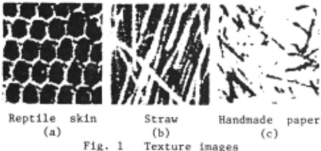
An input image is digitized into 64x64 pixels and is quantized into 64 gray levels. Fig. 1 shows digital images of three kinds of textures. Since input conditions may change the first order statistics of brightness distributions, the input image is normalized with respect to gray scale changes so that the mean of the brightness distribution is 32 and the standard deviation is B. Next, the normalized image is deblurred by an edge preserving averaging method to extract texture elements easily.
2.2 Extraction of Elements
A texture element is defined as a connected area with almost same gray levels. To extract such elements, pixels which are adjacent and whose gray levels are almost same are merged into regions. The merging process used here is as follows.
First, any pixels which are adjacent and whose gray level differences are less than the threshold d(=l) are merged into regions and their gray levels are averaged. Here, the total brightness change caused by averaging is examined. The total change is defined as
(x,y) whereod(x,y) is the gray level change at a ooint (x,y). Next, d is increased by one (d+d+l) and the merging process is repeated until one of the following conditions is satisfied (d>4).
- the total change is very large, which implies that d has become large enough to merge different elements, or
- the total change implies that there may between different kinds is very small, which be a brightness gap of elements.
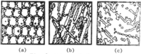
When the process stops at a threshold d* on the condition (1), the regions obtained by merging at d*-1 are used for the texture elements. When the process stops on the condition (2), the segmented region by thresholding the brightness histogram are used for the texture elements. For example, Fig. 2 shows the thus obtained elements of the images in Fig. 1.
2.3 Properties of Element
The following five kinds of properties are measured for each extracted element. They are used for global discrimination of elements.
- brightness
- area
(3) size
The size of an element is defined as 2 x area/perimeter. For example, when an element is a circle of radius r, the size is r. The value of this size descriptor is not affected greatly by overlap of individuals which may be extracted as one element on the image level.
(4) directionality (direction and magnitude) The directionality of an element is measured by the principal component analysis. The direction of the element is defined by the slope of the major axis. The magnitude D of the directionality is defined by the eigenvalues A1 and Az (Al~Az) of the covariance matrix for the distribution of (x,y) coordinates of points in the element, as
When an element is a circle, D=O. When an element is a straight line, 0=1.
(5) curvatures along the contour
In the distribution of curvatures along the contour of an element is meaningful information about the complexity of the shape. We measure the k-curvature (k=5) [5) at each contour point, Next, a measured curvature p is classified into six zones:
i) high concave curve: -75°<p<-45°
ii) low concave curve: -45°~p~-l5°
iii) straight line -l5°~p~ 15°
iv) low convex curve: 15°~< 45°
v) high convex curve: 45°~PI 75°
vi) zig-zag line the other
and the occurence probabilities of curvatures in the first five zones are calculated for the element properties,
2,4 Classification of Elements
On the basis of the distributions of these properties, elements are classified into some discriminable classes. In our system, elements are classified by thresholding the histogram of each property. In computing the histogram of a property, we use the weighted value as its frequency to give large weight to dominant elements. The weighting values are shown in Table 1. For example, the frequency of brightness b is defined as the total area (not number) of elements whose brightness are b. Therefore, the system can s~ably analyze a texture image in which there are comparatively small number of elements. Since each property has a different domain and range, the histogram is normalized and the thresholds are set automatically at the bottoms of deep valleys between the prominent peaks, if any [3].
2.5 Description of Texture
Statistical Features
Now, the system calculates the statistical features about elements class. following in each
(1) the number of classes: Nc
(2) the mean and the deviation of each property p of elements in each class i: (~ ,oi ) (i·l~Nc and pal~Np, where Np is the numS~r gf properties). The weighted values in Table 1 are also used for calculating these
| PROPERTY | WEIGHTING |
|---|---|
| BRIGHTNESS | AREA |
| SIZE | PERIMETER |
| AREA | AREA |
| DIRECTIONALITY .DIRECTION | AREA x MAGNITUDE |
| .MAGNITUDE | AREA |
| CURVATURES | PERIMETER |
distributions.
Furthermore, the following features concerning to placements of elements are easily measured. (3) the density of elements in each class i: Ai (i=l~Nc), which is the ratio of the total area of elements in class i to the image area.
(4) the adjacency probability between class i and class k: Pik (i,k·l~Nc), which is defined as the probability that a boundary point of an element in class i is adjacent to that in class k. When i =k, it is especially called 'auto-adjacency probability',
Table 2 shows the values of these textural features of the images in Fig. 1.
Figure and Ground
If there is more than one class of elements, one of them can be regarded as the "ground" of the image, The "ground" class is defined as
| ·- TEXTURE | (a) | -- (b) | (c) | |||||||||||||
|---|---|---|---|---|---|---|---|---|---|---|---|---|---|---|---|---|
| No. of class | ! 1 i | 2 | r 1 I I | -- 2 | 1 I | --r---------- 2 | ||||||||||
| properties | MEAN | S.D. | MEAN | S.D. | MEAN | I S.D. I I | MEAN | S.D. | - MEAN | ---··----+---· S.D. | MEAN | S.D. | ||||
| brightness | 19.2 | 5.2 | 36.1 | 1.4 | 18.5 | I 3,8 I | 35.0 | 2.4 | 27.0 | 0.2 | 45.4 | 2.9 | ||||
| size | 2.9 | 0.6 | 8.2 | 2.1 | 3.6 | 0.9 | 6.9 | 3.1 | 8.9 | 0.8 | 3.4 | 0.9 | ||||
| area | 12.9 | 11.7 | 73.3 | 70.0 | 32.6 | 36.2 | 67.4 | 175.2 | 2664.5 | /1)8.3 | 144.1 | 105.2 | ||||
| directionality .magnitude (%) | 56.6 | 26.5 | 34.3 | 24.4 | 78.8 | 28.0 | 71.4 | 22.7 | 7.0 | 6.9 | 28.7 | 29.0 | ||||
| .direction curvatures | 16.4 | 4.2 | 17.7 | 2.0 | 17.7 | 2.7 | 17.3 | 1.2 | 17.9 | 0.8 | 23.0 | 3.8 | ||||
| .[-75°,-45°] | (%) 4.4 | 6.1 | 5.3 | 4.5 | 1.9 | 3.5 | 4.4 | 3.2 | 9.6 | I 2.1: | 8.6 | 5.9 | ||||
| . [-45° ,-15°] | (%) 21.0 | 15.2 | 17.9 | 7.7 | 20.8 | 9.8 | 19.8 | 9.9 | 24.7 | 5.11 | 24.3 | 12 . 8 | ||||
| .[-15°, 15°] | (%) 13.9 | 13.4 | 16.0 | 8.3 | 32.6 | 17.5 | 32.1 | 16.1 | 28.8 | 5.6: | 22.8 | 13.7 | ||||
| .[ 15°, 45°] | (%) 24.4 | 22.1 | 36.2 13.3 | 31.4 | 17 . 5 | 24.5 | 12.8 | 23.7 | 8. 5: | 19.6 | 10.8 | |||||
| .[ 45°, 75°] | (%) 9.1 | 10.5 | 18.9 | 8.5 | 6.1 | 8,6 | 7.0 | 8.0 | 9.2 | 3.1: | 8.3 | 9.9 | ||||
| density | (%) | 30 | 70 | 29 | ____j_ | ___ | 7 1 73 | I 27 I . . ... | L___ ____ | _ | ||||||
| I 1 2 I | _1_ L | |||||||||||||||
| adjacency- probabilities (%) | 1 22 78 | 2 93 | 7 | ~ 1 0 2 | 0 | 11 0 100 2 97 3 | ||||||||||
- --
----------·
- a class whose average area of elements is very large (for example, class 1 of (c) in Table 2), otherwise,
- a class whose ratio of the deviation to the mean of areas of elements is very large (for example, class 2 of (b) in Table 2), otherwise,
- a class which has the largest auto-adjacency probability (for example, class 1 of (a) in Table 2).
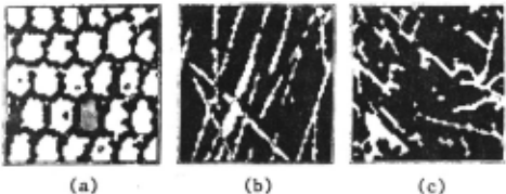
The other classes are in turn regarded as the "figures" .of the image, If the image has only one class of elements, it is regarded as both the "figure" and the "ground", For example, the "grounds" of the images in Fig, 1 are smeared with black as shown in Fig, 3.
Typical Element
The system selects one typical element from each "figure" class to give a detailed shape description of the elements in that class. The typical element in each "figure" class is the one whose shape properties are the closest to the means of those of that class, The function that evaluates the closeness of an element j in class i is defined as
where xjp is the value of a property p of an element j and the shape properties used are area, size, directionality and curvatures . For example, the dotted areas in Fig. 3 are the typical elements of the image in Fig, 1.
It is an important problem how a typical element is to be described for a detailed comparison needed in recognition phase of the system. There are many algorithms for shape analysis [6] and we should select a information preserving technique. In this paper, however, only the points in a typical element are memorized in terms of the relative coordinates from the centroid of the element for s implicity,
Relative Position Vectors
To give a detailed description also of placements of elements, the system measures relative positions among elements in "figure" classes. A relative position between two elements is defined as the relative coordinate between their centroids. The two dimentional histogram Hik of the relative positions of every pair of elements, one in class i and the other in class k (including i=k), are computed, Here, in computing the histogram '"e use the weighted value as its frequency as follows. Let Eij be the closeness of an element j in class i and Ekl be that of an element 1 in class k, Then the weighted value is defined as min(Eij,Ekl). If the placement is regular, there are significant clusters periodically in the histogram. In such a case, the mean and deviation of each independent cluster which is nearest to the origin is measured as the placement rule Rik, They are denoted as
where Nik is the number of independent clusters. If there is no significant cluster, the placement rule Rik is regarded as random.
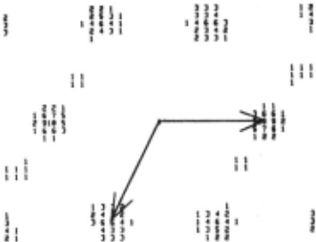
For example, Fig, 4 shows the distributions H22 of relative positions of elements in the "figure" class 2 of the !mage in Fig. l(a), In this case, the placement is regarded as regular and two independent clusters (whose means are (13,-6) and (0,11)) are measured, On the other hand, those of the other images in Fig, 1 are regarded as randam.
Now, the description of texture is completed, This description can be used for learning and recognition (classification) of texture images. Classification experiments using only the statistical features are reported in [3].
3. RECONSTRUCTION OF TEXTURES
The synthesis program in the system generates a texture image on the basis of the description of the original texture. It reconstructs a texture image so that the statistical features may be the same as those of the original one.
3.1 Modification£[ Typical Element
To reconstruct the texture elements, the system uses the typical element in each "figure" class and modi f ies it according to the distributions o~ the properties of elements in its class. The pr operties usee! for Mod5_fication are brightness (for light and darkness), size (for nagnificntion and reduction), direction (for rotation), and the !l'agnitude of directionality (for compres s ion).
For exaMple, let (~ip'crip) be the ncan and deviation of the proper ty p of elements in class i. The typical e lement is modified so that the distribution of a property p is N[~ip'O'ip] using a normal randon number gcnerater.
Nodified elements in such a way are then arranged according to the placement rules as mentioned .in the next section.
3.2 Placement of Modified Elements
The system determines the positions at uhich modified typical elements are placed as follows. If there are more than one "figure" class, one dominant "figure" class is selected. That is, the positions of::: .. elements of the dominant "figure" class (let it be now i) are at firRt determined according to the placement rule Rii and those of other class k are determined later according to Rik or Rkk. Our system defines a class i as the dominant one whose average deviation in the placement rule Rii is the smallest. The positions of elements in the dominant clas::; are determined as follows.
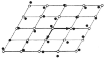
When the placement rule Rii is regular, the distributions of relative positions in Rii is used. First. the preliminary positions are determined using the means in Rii
as shown by white points in Fig. 5 (in this case 0 Nii·2). Next 0 these preliminary positions are fluctuated according to the normal distribution
·
as shown by black points in Fig. 5 using a normal random generator, where ax and O'y are the average deviations in Rii. These black points are the final positions at which modified elements are placed.
When the placement rule Rii is random. the system uses the density Ai of elements to determine the positions. Since the number of arranged elements is expected as
the system arranges such number of positions randomly over the image using a uniform random number generator.
Next 0 the position of elements in other class k(+i) are determined in almost the same way according to the placement rule Rik or Rkk.
Refering to thus determined positions. modified elements in each "figure" class are placed. After all the "figure" elements are placed 0 there remains blank space which corresponds to the "ground" of the image. It is filled up with gray values on the basis of the statistical features of the "ground" class by a region growing method.
Now. the reconstruction of texture is completed. Fig. 6 shows examples of the reconstructed images from the original ones in Fig. 1.
4. DISCUSSIONS
For our experiments. we used the same texture samples from Brodatz's photographic album [7] as used in classification (3]. The structural analysis produces anthropomorphic descriptions and therefore they are easily understandable and useful. problems by images. However, we found some important reconstructing those texture Since we only use brightness information to extract texture elements, they do not always correspond to real individuals or what human beings perceive. For example, overlapped individuals with same brightness are extracted as one element on the image level.
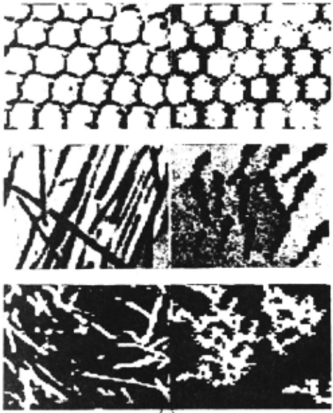
Also the "grounds" which the system selects do not always correspond to those which human beings select. This problem relates to the definition of elements,
The placement rules used (relative positions) is the second order statistics and may be still too simple. For example, though the position of an element is considered independently of its properties and those of surrounding elements, there are often correlations among them,
In this paper, we hardly deal with hierarchical textures. A hierarchical texture is such that a set of several elements can be regarded as a unit and many such units are arranged according to their own placement rules. Such hierarchical textures, however, are more often found in artificial textures. If we add aggregation programs [8] to our system, we would be able to describe them in the same way,
ACKNOl-TLEDGEMENT
The authors wish to express their thanks to members of the Computer Vision Research Section, Electrotechnical Laboratory, for their kind help.
@inproceedings{ijcai1979p195,
  title     = {Description of Textures by a Structural Analysis},
  author    = {Tomita, Fumiaki and Shirai, Yoshiaki and Tsuji, Saburo},
  booktitle = {Proceedings of the Sixth International Joint Conference on
               Artificial Intelligence, {IJCAI-79}},
  publisher = {International Joint Conferences on Artificial Intelligence},
  editor    = {Bruce G. Buchanan},
  year      = {1979},
  month     = {8},
  url       = {https://ijcai.org/proceedings/1979/195},
}
TY - CPAPER TI - Description of Textures by a Structural Analysis AU - Tomita, Fumiaki AU - Shirai, Yoshiaki AU - Tsuji, Saburo T2 - Proceedings of the Sixth International Joint Conference on Artificial Intelligence, IJCAI-79 PB - International Joint Conferences on Artificial Intelligence PY - 1979 UR - https://ijcai.org/proceedings/1979/195 ER -Copied
Machine-readable versions of this paper, for tools and AI agents:





