
Semifactual Explanations for GNN-based Classification: Formal Foundations, Complexity and Computation
Proceedings of the Thirty-Fifth International Joint Conference on Artificial Intelligence. Main Track. Pages 4125-4134.
https://doi.org/10.24963/ijcai.2026/459
Keywords
- Machine Learning: Explainable/Interpretable machine learning
Abstract
Graph Neural Networks (GNNs) have become increasingly central to several analysis tasks in various domains, ranging, e.g., from social networks to molecular analysis. Understanding the decision-making process of GNNs is a critical challenge in machine learning, particularly when post-hoc explanations, attempting to answer why specific inputs are classified in a certain way by a given model, are required for specific input predictions. Existing post-hoc explainability methods for GNNs often rely on counterfactual reasoning, grounded in the `if this had not occurred' thinking, that typically identifies minimal subgraphs perturbations that would change a prediction. Notably, less attention has been posed on the equally important semifactual reasoning, grounded in the `even if this has not occurred' thinking, that results in identifying maximal subgraphs perturbations that would not change a prediction. In this paper, we introduce a novel technique for post-hoc explainability queries in GNNs by focusing on the semifactual reasoning. We first thoroughly investigate the computational complexity of several reasoning and optimization problems related to the computation of semifactuals, and then propose a novel learning architecture for addressing their computation. Finally, we experimentally evaluate the proposed approach in a variety of settings, showing its effectiveness in generating high-quality semifactual explanations.
- [Alfano et al., 2024] Gianvincenzo Alfano, Sergio Greco, Francesco Parisi, and Irina Trubitsyna. Counterfactual and semifactual explanations in abstract argumentation: Formal foundations, complexity and computation. In Proceedings of International Conference on Principles of Knowledge Representation and Reasoning (KR), pages 14-26, 2024.
- [Alfano et al., 2025a] Gianvincenzo Alfano, Adam Gould, Francesco Leofante, Antonio Rago, and Francesca Toni. Counterfactual explanations under model multiplicity and their use in computational argumentation. In Proceedings of International Joint Conference on Artificial Intelligence (IJCAI), pages 4321-4329. ijcai.org, 2025. IJCAI
- [Alfano et al., 2025b] Gianvincenzo Alfano, Sergio Greco, Domenico Mandaglio, Francesco Parisi, Reza Shahbazian, and Irina Trubitsyna. Decentralized federated learning meets physics-informed neural networks. Knowledge- Based Systems, 323:113717, 2025.
- [Alfano et al., 2025c] Gianvincenzo Alfano, Sergio Greco, Domenico Mandaglio, Francesco Parisi, Reza Shahbazian, and Irina Trubitsyna. Even-if explanations: Formal foun- dations, priorities and complexity. In Proceedings of the AAAI Conference on Artificial Intelligence, volume 39, pages 15347-15355, 2025.
- [Allamanis et al., 2018] Miltiadis Allamanis, Earl T Barr, Premkumar Devanbu, and Charles Sutton. A survey of machine learning for big code and naturalness. ACM Com- puting Surveys (CSUR), 51(4):1-37, 2018.
- [Arenas et al., 2021] Marcelo Arenas, Daniel Baez, Pablo Barceló, Jorge Pérez, and Bernardo Subercaseaux. Foun- dations of symbolic languages for model interpretability. Proceedings of Advances in Neural Information Process- ing Systems, 34:11690-11701, 2021.
- [Arenas et al., 2022] Marcelo Arenas, Pablo Barceló, Miguel Romero Orth, and Bernardo Subercaseaux. On computing probabilistic explanations for decision trees. Proceedings of Advances in Neural Information Processing Systems, 35:28695-28707, 2022.
- [Arora and Barak, 2009] Sanjeev Arora and Boaz Barak. Computational Complexity -A Modern Approach. Cam- bridge University Press, 2009.
- [Artelt et al., 2025] André Artelt, Martin Olsen, and Kevin Tierney. On the hardness of computing counterfactual and semi-factual explanations in XAI. Transactions on Ma- chine Learning Research, 2025.
- [Aryal and Keane, 2023] Saugat Aryal and Mark T. Keane. Even if explanations: Prior work, desiderata & bench- marks for semi-factual xai. In Proceedings of Interna- tional Joint Conference on Artificial Intelligence (IJCAI), pages 6526-6535, 2023. IJCAI
- [Azzolin et al., 2025] Steve Azzolin, Sagar Malhotra, An- drea Passerini, and Stefano Teso. Beyond topological self-explainable gnns: A formal explainability perspective. In Proceedings of International Conference on Machine Learning (ICML), pages 2045-2080, 2025.
- [Barceló et al., 2020] Pablo Barceló, Mikaël Monet, Jorge Pérez, and Bernardo Subercaseaux. Model interpretabil- ity through the lens of computational complexity. In Pro- ceedings of Advances in Neural Information Processing Systems, 2020.
- [Bassan et al., 2025] Shahaf Bassan, Ron Eliav, and Shlomit Gur. Explain yourself, briefly! self-explaining neural net- works with concise sufficient reasons. In Proceedings of International Conference on Learning Representations, 2025.
- [Borgwardt et al., 2005] Karsten M Borgwardt, Cheng Soon Ong, Stefan Schönauer, SVN Vishwanathan, Alex J Smola, and Hans-Peter Kriegel. Protein function predic- tion via graph kernels. Bioinformatics, 21(suppl 1):i47- i56, 2005.
- [Calautti et al., 2025] Marco Calautti, Enrico Malizia, and Cristian Molinaro. On the complexity of global necessary reasons to explain classification. In Proceedings of Inter- national Conference on Principles of Knowledge Repre- sentation and Reasoning (KR), pages 206-217, 2025.
- [Cho et al., 2011] Eunjoon Cho, Seth A Myers, and Jure Leskovec. Friendship and mobility: user movement in location-based social networks. In Proceedings of ACM SIGKDD International Conference on Knowledge Discov- ery and Data Mining, pages 1082-1090, 2011.
- [Dandl et al., 2023] Susanne Dandl, Giuseppe Casalicchio, Bernd Bischl, and Ludwig Bothmann. Interpretable re- gional descriptors: Hyperbox-based local explanations. In Proceedings of Machine Learning and Knowledge Dis- covery in Databases, volume 14171, pages 479-495. Springer, 2023.
- [Debnath et al., 1991] Asim Kumar Debnath, Rosa L Lopez de Compadre, Gargi Debnath, Alan J Shusterman, and Corwin Hansch. Structure-activity relationship of mutagenic aromatic and heteroaromatic nitro compounds. correlation with molecular orbital energies and hydropho- bicity. Journal of medicinal chemistry, 34(2):786-797, 1991.
- [Eiben et al., 2023] Eduard Eiben, Sebastian Ordyniak, Gia- como Paesani, and Stefan Szeider. Learning small decision trees with large domain. In Proceedings of International Joint Conference on Artificial Intelligence (IJCAI), pages 3184-3192, 2023. IJCAI
- [El Harzli et al., 2023] Ouns El Harzli, Bernardo Cuenca Grau, and Ian Horrocks. Cardinality-minimal explanations for monotonic neural networks. In Proceedings of Interna- tional Joint Conference on Artificial Intelligence (IJCAI), pages 3677-3685, 2023. IJCAI
- [Guidotti, 2024] Riccardo Guidotti. Counterfactual expla- nations and how to find them: literature review and benchmarking. Data Mining and Knowledge Discovery, 38(5):2770-2824, 2024.
- [Guo et al., 2025] Zhimeng Guo, Zongyu Wu, Teng Xiao, Charu Aggarwal, Hui Liu, and Suhang Wang. Counterfac- tual learning on graphs: A survey. Machine Intelligence Research, 22(1):17-59, 2025.
- [Huang et al., 2023] Zexi Huang, Mert Kosan, Sourav Me- dya, Sayan Ranu, and Ambuj Singh. Global counterfactual explainer for graph neural networks. In Proceedings of the Sixteenth ACM International Conference on Web Search and Data Mining, pages 141-149, 2023.
- [Ignatiev et al., 2019] Alexey Ignatiev, Nina Narodytska, and João Marques-Silva. Abduction-based explanations for machine learning models. In Proceedings of AAAI Conference on Artificial Intelligence, pages 1511-1519, 2019.
- [Ignatiev et al., 2022] Alexey Ignatiev, Yacine Izza, Peter J. Stuckey, and João Marques-Silva. Using maxsat for ef- ficient explanations of tree ensembles. In Proceedings of AAAI Conference on Artificial Intelligence, pages 3776- 3785, 2022.
- [Ivanov et al., 2019] Sergei Ivanov, Sergei Sviridov, and Evgeny Burnaev. Understanding isomorphism bias in graph data sets. arXiv preprint arXiv:1910.12091, 2019.
- [Kenny and Huang, 2023] Eoin M. Kenny and Weipeng Huang. The utility of "even if" semi-factual explanation to optimise positive outcomes. In Thirty-seventh Confer- ence on Neural Information Processing Systems, 2023.
- [Kenny and Keane, 2021] Eoin M Kenny and Mark T Keane. On generating plausible counterfactual and semi-factual explanations for deep learning. In Proceedings of AAAI Conference on Artificial Intelligence, pages 11575-11585, 2021.
- [Kipf and Welling, 2016] Thomas N Kipf and Max Welling. Semi-supervised classification with graph convolutional networks. arXiv preprint arXiv:1609.02907, 2016.
- [Kosan et al., 2024] Mert Kosan, Samidha Verma, Burouj Armgaan, Khushbu Pahwa, Ambuj Singh, Sourav Medya, and Sayan Ranu. Gnnx-bench: Unravelling the utility of perturbation-based gnn explainers through in-depth bench- marking. In International Conference on Learning Repre- sentations, 2024.
- [Lin et al., 2021] Wanyu Lin, Hao Lan, and Baochun Li. Generative causal explanations for graph neural networks. In International Conference on Machine Learning, pages 6666-6679. PMLR, 2021.
- [Luo et al., 2020] Dongsheng Luo, Wei Cheng, Dongkuan Xu, Wenchao Yu, Bo Zong, Haifeng Chen, and Xiang Zhang. Parameterized explainer for graph neural net- work. Advances in Neural Information Processing Sys- tems, 33:19620-19631, 2020.
- [Malfa et al., 2021] Emanuele La Malfa, Rhiannon Michel- more, Agnieszka M. Zbrzezny, Nicola Paoletti, and Marta Kwiatkowska. On guaranteed optimal robust explanations for NLP models. In Proceedings of International Joint Conference on Artificial Intelligence (IJCAI), pages 2658- 2665, 2021. IJCAI
- [Marques-Silva and Ignatiev, 2022] João Marques-Silva and Alexey Ignatiev. Delivering trustworthy AI through for- mal XAI. In Proceedings of AAAI Conference on Artificial Intelligence, pages 12342-12350, 2022.
- [Marzari et al., 2023] Luca Marzari, Davide Corsi, Ferdi- nando Cicalese, and Alessandro Farinelli. The #dnn- verification problem: Counting unsafe inputs for deep neu- ral networks. In Proceedings of International Joint Con- ference on Artificial Intelligence (IJCAI), pages 217-224, 2023.
- [Ordyniak et al., 2023] Sebastian Ordyniak, Giacomo Pae- sani, and Stefan Szeider. The parameterized complexity of finding concise local explanations. In Proceedings of In- ternational Joint Conference on Artificial Intelligence (IJ- CAI), pages 3312-3320, 2023. IJCAI
- [Prado-Romero et al., 2024a] Mario Alfonso Prado- Romero, Bardh Prenkaj, and Giovanni Stilo. Robust stochastic graph generator for counterfactual explana- tions. In Proceedings of the AAAI Conference on Artificial Intelligence, pages 21518-21526, 2024.
- [Prado-Romero et al., 2024b] Mario Alfonso Prado- Romero, Bardh Prenkaj, Giovanni Stilo, and Fosca Giannotti. A survey on graph counterfactual explanations: definitions, methods, evaluation, and research challenges. ACM Computing Surveys, 56(7):1-37, 2024.
- [Riesen and Bunke, 2008] Kaspar Riesen and Horst Bunke. Iam graph database repository for graph based pattern recognition and machine learning. In Structural, Syntactic, and Statistical Pattern Recognition: Joint IAPR Interna- tional Workshop, SSPR & SPR 2008, Orlando, USA, De- cember 4-6, 2008. Proceedings, pages 287-297. Springer, 2008.
- [Tan et al., 2022] Juntao Tan, Shijie Geng, Zuohui Fu, Yingqiang Ge, Shuyuan Xu, Yunqi Li, and Yongfeng Zhang. Learning and evaluating graph neural network ex- planations based on counterfactual and factual reasoning. In Proceedings of the ACM Web Conference, pages 1018- 1027, 2022.
- [Verma et al., 2024] Samidha Verma, Burouj Armgaan, Sourav Medya, and Sayan Ranu. Induce: Inductive coun- terfactual explanations for graph neural networks. Trans- actions on Machine Learning Research, 2024.
- [Wale et al., 2008] Nikil Wale, Ian A Watson, and George Karypis. Comparison of descriptor spaces for chemical compound retrieval and classification. Knowledge and In- formation Systems, 14:347-375, 2008.
- [Xie et al., 2022] Yaochen Xie, Sumeet Katariya, Xianfeng Tang, Edward Huang, Nikhil Rao, Karthik Subbian, and Shuiwang Ji. Task-agnostic graph explanations. Advances in Neural Information Processing Systems, 35:12027- 12039, 2022.
- [Ying et al., 2019] Zhitao Ying, Dylan Bourgeois, Jiaxuan You, Marinka Zitnik, and Jure Leskovec. Gnnexplainer: Generating explanations for graph neural networks. Ad- vances in Neural Information Processing Systems, 32, 2019.
- [You et al., 2018] Jiaxuan You, Bowen Liu, Zhitao Ying, Vi- jay Pande, and Jure Leskovec. Graph convolutional pol- icy network for goal-directed molecular graph generation. Advances in Neural Information Processing Systems, 31, 2018.
- [Yuan et al., 2021] Hao Yuan, Haiyang Yu, Jie Wang, Kang Li, and Shuiwang Ji. On explainability of graph neural net- works via subgraph explorations. In International Confer- ence on Machine Learning, pages 12241-12252. PMLR, 2021.
- [Yuan et al., 2022] Hao Yuan, Haiyang Yu, Shurui Gui, and Shuiwang Ji. Explainability in graph neural networks: A taxonomic survey. IEEE Transactions on Pattern Analysis and Machine Intelligence, 45(5):5782-5799, 2022.
- [Zhang et al., 2022] Shichang Zhang, Yozen Liu, Neil Shah, and Yizhou Sun. Gstarx: Explaining graph neural net- works with structure-aware cooperative games. In Ad- vances in Neural Information Processing Systems, 2022.
- [Zitnik et al., 2018] Marinka Zitnik, Monica Agrawal, and Jure Leskovec. Modeling polypharmacy side effects with graph convolutional networks. Bioinformatics, 34(13):i457-i466, 2018.
References were extracted automatically from the PDF and may contain errors.
Full text extracted automatically from the PDF; figures, tables and equations may differ. The PDF is the version of record.
1 Introduction
Graph-structured data, where entities (nodes) are related by pairwise relationships (edges), play a central role in machine learning applications, arising naturally in domains such as molecular property prediction, social network analysis, and recommendation systems [Cho et al., 2011; You et al., 2018; Zitnik et al., 2018]. In these settings, Graph Neural Networks (GNNs) have emerged as the leading models for predictive tasks on graphs. Despite their predictive power, understanding and explaining GNNs decision-making remains a fundamental challenge, especially in high-stakes applications where trust, transparency, and robustness are essential.
Post-hoc GNN explanation methods aim to shed light on why a model assigns a particular prediction at the graph, node, or edge level [Yuan et al., 2022]. These methods typically provide either factual explanations, identifying the most relevant subgraph or node features supporting the model's decision, or counterfactual explanations [Prado-Romero et al., 2024b], which ask how minimal graph changes-e.g., adding or deleting a few edges-could alter the model's decision.
However, less attention has been devoted to an equally important and complementary paradigm, namely, semifactual 'even-if' reasoning [Aryal and Keane, 2023; Kenny and Huang, 2023; Alfano et al., 2024]. While semifactual explanations have been explored in other settings-such as models operating on tabular or binary data [Aryal and Keane, 2023; Alfano et al., 2025c; Kenny and Huang, 2023]-this paradigm has not yet been investigated for graph-structured data or GNNs [Artelt et al., 2025]. In contrast to counterfactual explanations, which focus on identifying minimal changes that would alter a model's prediction [Prado-Romero et al., 2024a], semifactual explanations seek to identify the largest perturbations to the graph structure that leave the prediction unchanged. This kind of explanation is particularly useful when predictions correspond to positive or desired outcomes, as it reveals the robustness of the model's decision and uncovers degrees of freedom in the input that do not affect the outcomes [Alfano et al., 2025c]. Indeed, the greater the number of perturbations captured by the semifactual explanation, the more informative and convincing the explanation becomes [Aryal and Keane, 2023]. Intuitively, this reflects a user's desire to understand the extent of variation and favorable conditions that can be tolerated while keeping a positive status assigned by the model.
Consider the following example from molecular property prediction, where semifactual reasoning can help identify molecular perturbations that preserve desired properties.
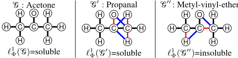
Example 1. Consider a scenario where graphs model molecules, that is where nodes correspond to atoms, edges to links between them, and node features represent intrinsic properties of atoms (e.g., atomic number, mass number, etc.). Assume that a GNN Φ has been trained to predict the watersolubility of molecules. 1 Consider the graph G (shown in Figure 1 (left)) representing Acetone, whose molecular formula is C3H6O, and whose (first most probable class) label is ℓ1Φ(G) = 'soluble' meaning that Acetone is water-soluble. To explain Φ under the semifactual reasoning, we would like to know the 'farthest' molecule w.r.t. Acetone that has the same atoms (thus the same molecular formula) and is still classified as water-soluble from GNN Φ. Thus, a semifactual for Gw.r.t. Φ could be G′ that represents Propanal-a structural isomer of Acetone 2 -obtained from Gwith 6 modifications (3 deletions and 3 additions, respectively shown as red and blue edges in Figure 1 (center)). Conversely, under counterfactual reasoning, we would like to know the 'closest' structural isomer no longer classified as water-soluble from Φ. A counterfactual for Gw.r.t. Φ could be G′′ , that is, Methylvinyl-ether, obtained from Gwith 4 modifications (see Figure 1 (right)). ✷
1 A molecule is water-insoluble if having a Henry's Law constant greater than 10-3 atm-cu m/mole; water-soluble otherwise.
Semifactual explanations for graph-structured data have potential relevance across multiple domains, e.g., identifying stable user-item interactions in recommendation systems or supporting the assessment of prediction resilience in traffic and social networks. Nevertheless, to the best of our knowledge, semifactual reasoning for GNNs or graph-structured learning tasks has not been explored so far.
Contributions. Our main contributions are as follows.
- We formally introduce the concept of semifactual explanations for graph (and node) classification tasks in GNN models (Section 3), showing that semifactual explanations generalize factual ones [Tan et al., 2022; Ying et al., 2019; Lin et al., 2021; Luo et al., 2020; Yuan et al., 2021].
- We investigate the computational complexity of natural semifactual-based reasoning problems for graph (and node) classification tasks in GNN models (Section 4). It turns out that semifactual-based problems are as challenging as their counterfactual counterparts. In this regard, we strengthen the characterization of the computational complexity of some counterfactual-based problems fromNPhardness to FPNP[log n] -completeness.
- Motivated by the fact that above mentioned problems are computationally costly (particularly, FPNP[log n] -hard), we introduce a learning architecture for the heuristic computation of semifactuals. In our approach, semifactual explanations are computed by finding the parameters of a
2 Molecules sharing the formula and differing in the connectivity of their carbon atoms are called structural isomers.
- neural network model (see Figure 2 for an overview) that minimizes a loss function and enforces the desired properties of semifactuals (Algorithm 1).
- We empirically evaluate the proposed learning architecture in several widely used benchmark datasets for graph classification (Section 6). An ablation analysis confirms that all modules included in our architecture positively contribute to effectiveness in computing semifactuals. Our method is competitive also in the factual setting, outperforming or matching methods tailored to the factual setting.
Reproducibility. For the sake of reproducibility, all our code and the datasets used in this paper are available at https://github.com/Ralyhu/semifactual-gnn.
2 Preliminaries
We represent an attributed undirected graph (AUG) as G= (V,E,X), where V = {1, 2, . . . , n} is the set of nodes, E ⊆ V × V is the set of edges such that (u, v) ∈ E implies (v, u) ∈ E, and X ∈ Rn×d = [xu ∈ Rd ]u∈V is the matrix of node features. Herein, each vector xu ∈ Rd encodes intrinsic properties of node u ∈ V . For each node u ∈ V , we use N(u) to denote the set of its neighbors, that is, N(u) = {v ∈ V | (u, v) ∈ E}. We denote the graph's adjacency matrix as A ∈ {0, 1}n×n , where Auv = Avu = 1 if there is an edge connecting u and v; otherwise, Auv = Avu = 0. Hereafter, given a graph G= (V, E, X) and a set E′ ⊆ E of edges, we use G′ = (V, E′ ,X) to denote the subgraph of Gwhere only the edges in E′ are considered. With a little abuse of notation, we also use G= (A, X) to denote G= (V, E, X), where A is the adjacency matrix of (V, E).
Given an AUG G= (V,E,X), with node features xu ∈ Rd for each u ∈ V , a GNN Φ learns node representations of each node u by iteratively aggregating information from nodes' neighbors N(u). A layer in a GNN defines a transformation step where node representations are updated based on their own features and those of their neighbors. Starting with h(0) u = xu, the representation of node u at the i-th GNN layer, denoted by h(i) u , is updated as h(i) u = update(h(i-1) u , h(i) N(u) ), where h(i-1) u is the previous layer's representation of u and h(i) N(u) is an aggregated representation of its neighbors, computed as h(i) N(u) = aggregate(h(i-1) v | v ∈ N(u)). Here, aggregate(·) collects information from the neighbors, and update(·) combines it with the current node's representation. The specific implementations of update(·) and aggregate(·) functions vary across different GNN models. In a GNN with κ layers, the final representation of a node u is given by h(κ) u . Once the node representations have been computed, an overall graph-level representation h(κ) G ∈ Rd′ (for some κ, d′ ∈ N) is typically obtained by pooling (e.g., averaging or summing) the node representations in the graph. We assume d′ = d, though our results hold even if d′ ̸= d. We also use the term graph (resp., node) embedding to refer to h(κ) G (resp., h(κ) u ), and simply denote it with Φ(G) (resp., Φ(G, u)). The computed graph embedding (resp., node embeddings) can subsequently be leveraged for various downstream prediction tasks such as graph (resp., node) classification. Specifically, in the graph (resp., node) classification task, the embedding Φ(G) (resp., Φ(G, u)) is used to compute a predicted graph label ˆ yG ∈ C (resp., node label ˆ yu ∈ C), where C denotes the set of class labels. We assume the existence of a trained GNN Φ, which has been optimized in a supervised fashion using a training set of labeled instances. The training process involves minimizing a suitable loss function (e.g., cross-entropy) between predicted and true labels, depending on the specific prediction task. In the graph classification setting, the GNN is trained over a collection of labeled graphs (each associated with a class label in C) while, in the node classification setting, the GNN Φ is trained on a graph where a subset of nodes has known labels. For any graph G, GNN Φ produces a (discrete) probability distribution P over the set of class labels; we use P(ˆ y G = c | Φ(G)) to denote the probability that Gbelongs to c ∈ C w.r.t. Φ. Moreover, we use ℓ1Φ(G) = argmaxc∈C P(ˆ y G = c | Φ(G)) and ℓ2Φ(G) = argmaxc∈(C\ℓ1Φ (G)) P(ˆ y G = c | Φ(G)) to denote the first and second-most probable class labels for G w.r.t. Φ, respectively. For the node classification task, we use P (ˆ yu = c | Φ(G, u)) to denote the probability that node u belongs to class c w.r.t. GNN Φ. The first and secondmost probable class labels for node u w.r.t. Φ is denoted by ℓ1Φ(G, u) and ℓ2Φ(G, u), respectively.
3 Semifactual Explanations for GNNs
In this section, we introduce semifactual explanations for the considered classification tasks. Intuitively, an explanation is a graph obtained from the input one by performing as many perturbations (i.e., edge additions and deletions) as possible, while keeping the same class label.
Hereafter, given two AUGs G = (V,E,X) and G′ = (V,E′ ,X), we adopt as distance between them the cardinality of the symmetric difference between their sets of edges E and E′ . That is, the distance between Gand G′ is defined as |E∆E′ | = |(E \ E′ ) ∪ (E′ \ E)|. The symmetric difference distance provides a natural and intuitive metric for capturing the number of modifications required to alter the system's output. It is commonly adopted in several works within explainable AI to compare vectors of (binary) features [Barcel´o et al., 2020; Guidotti, 2024]. Moreover, it ensures a balanced behavior between edge additions and deletions.
Often, in real-world contexts, only some changes on the original graph G(V, E, X) are possible. To this end, we use a perturbation set Ep ⊆ V ×V to represent the set of allowed perturbations. Although, our notion of perturbation set is not able to capture all kinds of allowed perturbations in any realworld system, e.g., those subjected to particular conditions such as the existence of an edge conditioned to some structural property of the graph, it enables explanations with the so-called actionability property by design [Guidotti, 2024].
We can now formally define semifactual explanations.
Definition 1 (Semifactual Explanations for Graph Classification). Let G = (V,E,X) be an AUG, Φ a GNN, and Ep ⊆ V × V a perturbation set. A Semifactual Explanation for Gw.r.t. Φ is a graph G′ = (V,E′ ,X) such that i) ℓ1Φ(G′ ) = ℓ1Φ(G), ii) (E∆E′ ) ⊆ Ep , and iii) there is no G′′ = (V,E′′ ,X) with |E∆E′′ | > |E∆E′ | such that conditions i) and ii) hold.
Clearly, whenever Ep ⊆ E (resp., Ep ∩E = ∅) semifactual explanations consist of only deletions (resp., additions).
Example 2. In our running example, where Acetone is represented by the graph G= (V, E, X) of Figure 1 (left), the perturbation set Ep = {(u, v) ∈ V ×V | u or v is a carbon atom} naturally encodes the fact that structural isomers differ only in the relationships involving carbon atoms. As a result, we have that Propanal, represented by the graph G′ = (V,E′ ,X) in Figure 1 (center), is a semifactual for G(Acetone) w.r.t. the considered GNN at distance |E∆E′ | = 6. ✷
Relationships with factual explanations. Factual explanations have been proposed to offer insights into the reasoning behind a specific prediction by identifying the smallest subgraphs that can independently produce the same prediction as the full input graph [Tan et al., 2022; Ying et al., 2019; Lin et al., 2021; Luo et al., 2020; Yuan et al., 2021; Xie et al., 2022; Azzolin et al., 2025]. Using our notation, factual explanations can be formulated as follows.
Definition 2 (Factual Explanations for Graph Classification). Let G = (V,E,X) be an AUG, and Φ a GNN. A Factual Explanation for Gw.r.t. Φ is a graph G′ = (V,E′ ,X) such that i) ℓ1Φ(G′ ) = ℓ1Φ(G), ii) E′ ⊆ E, and iii) there is no G′′ = (V,E′′ ,X) with |E′′ | < |E′ | such that conditions i) and ii) hold.
We use SΦ(G) and FΦ(G) to denote the set of semifactual and factual explanations for Gw.r.t. Φ, respectively.
It is worth noting that, as stated in the following proposition, semifactual explanations generalize factual explanations. Briefly put, factual explanations are semifactual explanations where only edge deletions are allowed.
Proposition 1. For any AUG G= (V,E,X) and GNN Φ, it holds that FΦ(G)=SΦ(G) if Ep=E.
Node classification. Semifactual explanations for node classification can be defined analogously to Definition 1, where the focus is on graph classification. The only differences are i) a target node v we ask the explanation for is also given in input, and ii) ℓ1Φ(·) is replaced with ℓ1Φ(·, v).
4 Computational Complexity
We first explore the computational complexity of problems related to semifactual reasoning for graph classification. To provide a thorough analysis, we extend our investigation to related problems concerning counterfactual reasoning for graph classification, as well as to semifactual and counterfactual reasoning for node classification.
We start by investigating the complexity of two natural problems concerning semifactual reasoning for graph classification. The first problem asks whether there is a perturbed graph whose predicted label is that of the original one and having distance greater than or equal to a given threshold k. We call this problem decision-Semifactual reasoning for Graph classification (d-SG for short).
Definition 3 (d-SG). Let G = (V,E,X) be an AUG, Φ a GNN, k ∈ N an integer, and Ep ⊆ V × V a perturbation set. d-SG is the problem of checking whether there exists G′ = (V,E′ ,X) such that ℓ1Φ(G′ ) = ℓ1Φ(G), (E∆E′ ) ⊆ Ep and |E∆E′ | ≥ k.
| SEMIFACTUAL (X=S) | COUNTERFACTUAL (X=C) | |
|---|---|---|
| d-xG | NP-c [Thm. 1] | NP-c [Thm. 3] |
| Graph xG | FPNP[log n]-c [Thm. 2] | FPNP[log n]-c [Thm. 3] |
| Node d-xN | NP-c [Thm. 4] | NP-c [Thm. 4] |
| xN | FPNP[log n]-c [Thm. 4] | FPNP[log n]-c [Thm. 4] |
Deciding d-SG helps understanding whether a semifactual at a distance greater than or equal to k exists. Hence, it can be used to iteratively explore the space of candidate semifactuals in search of an optimal solution. Unfortunately, as stated next, even deciding d-SG is hard.
The second problem considered is the (functional) problem of computing a semifactual. We call this problem Semifactual reasoning for Graph classification (SG).
Definition 4 (SG). Let G = (V,E,X) be an AUG, Φ a GNN, and Ep ⊆ V ×V a perturbation set. SG is the problem of finding a graph G∗ = (V, E∗ , X) such that:
It is worth mentioning that, in computational complexity theory [Arora and Barak, 2009], d-SG is the so-called decision version of SG.
The result of Theorem 1 entails that SG is NP-hard. The following theorem provides a tight characterization of the complexity of finding semifactual explanations.
A natural question is whether semifactual explanations are harder to compute than counterfactual ones. Counterfactuals are defined as the minimal changes to apply to a given instance to let the prediction of the model be different [Barcel´o et al., 2020]. Problem d-CG (decision-Counterfactual reasoning for Graph classification) can be defined analogously to d-SG but by requiring different predicted labels and an upper-bound threshold.
Definition 5 (d-CG). Let G = (V,E,X) be an AUG, Φ a GNN, k ∈ N an integer, and Ep ⊆ V × V a perturbation set. d-CG is deciding whether there is a graph G′ = (V,E′ ,X) s.t. ℓ1Φ(G′ ) ̸= ℓ1Φ(G), (E∆E′ ) ⊆ Ep and |E∆E′ | ≤ k.
The problem of computing counterfactual explanations has been previously defined for node classification in [Verma et al., 2024]. Next, we introduce the Counterfactual reasoning for Graph classification (CG) problem.
Definition 6 (CG). Let G = (V,E,X) be an AUG, Φ a GNN, and Ep ⊆ V ×V a perturbation set. CG is the problem of finding a graph G∗ = (V, E∗ , X) such that:
As stated next, the complexity of counterfactual reasoning problems is the same as that of semifactual ones.
Theorem 3. d-CG is NP-complete. Moreover, CG is FPNP[log n] -complete.
The problems concerning semifactual and counterfactual reasoning for node classification (denoted as d-SN, SN, dCN, and CN) can be defined by mirroring those for graph classification: an additional target node v ∈ V is given as input, and ℓ1Φ(·) is replaced with ℓ1Φ(·, v). Notably, the complexity of CN has been studied in [Verma et al., 2024], where it is shown that CN is NP-hard. Here, we provide a tighter characterization of the complexity of CN. Moreover, we characterize the complexity of the other problems related to semifactual and counterfactual reasoning for node classification.
Theorem 4. d-SN and d-CN are NP-complete. Moreover, SN and CN are FPNP[log n] -complete.
The results of Theorems 2-4, summarized in Table 1, suggest that effective heuristics should be devised for the efficient computation of semifactual explanations.
5 Computation
We propose a neural approach to solve the SG problem (Definition 4). The adoption of a learning-based architecture is motivated the computational intractability of exact semifactual computation (cf. Section 4). This is in line with counterfactual problems that share the same complexity of semifactuals (cf. Thm. 2-3) and are mostly solved by learningbased approaches [Prado-Romero et al., 2024b]. Following the bulk of the literature on perturbation-based counterfactual explanations [Guo et al., 2025], we model an explanation as a mask matrix M ∈ [-1, 1]n×n , where |Muv| represents (during computation) the probability that edge (u, v) is added or removed. Consistently with this notation, we use (A,X) to denote an AUG G. Moreover, we use P ∈ {-1, 0, 1}n×n to denote the perturbation matrix, that is the matrix representation of the perturbation set Ep . In particular, P encodes the perturbations that might be applied to the adjacency matrix A in constructing semifactual explanations, as detailed next:
A semifactual explanations for (A,X) will be computed as (A∗ = round(A+M),X), where round(A+M) is the matrix obtained from A+M by rounding each element from [0, 1] to the closest value in {0, 1}. That is, A∗uv = 1 with Puv = 1 (resp., A∗uv = 0 with Puv = -1) means that edge (u, v) has been added (resp., deleted) to build a semifactual explanation. In all the other cases, it holds that Auv =A∗uv .
We propose a learning-based approach to find the best mask matrix M. We let a neural-network model fθ (with parameters θ) produce the mask matrix, thereby producing the semifactual explanations. The ultimate goal is to find the model parameters θ that minimizes a loss function that enforces the desired properties of the semifactuals, e.g., keeping the same predicted class. Leveraging a neural network model to generate the semifactual explanations, rather than treating them as trainable parameters, offers several advantages, e.g., it reduces the number of trainable parameters and allows us to exploit the graph topology to guide the generation of the mask. The proposed neural approach, termed SEMIX, is illustrated in its main components in Figure 2.

Neural model. Our fθ model takes as input a graph G = (A,X) and employs two parallel branches, each computing a mask matrix for each kind of edge perturbation: one for insertions, generating M+, and one for deletions, generating M-. We use M± (with ± ∈ {+,-}) to denote these mask matrices. In each of these branches, the first block of fθ consists of a (κ-layer) GNN Φ± having parameters θΦ± (see light-grey colored boxes in Figure 2). The two GNNs separately process the topology of Gand the matrix of node features X, producing node-level hidden representations. Specifically, each GNN outputs a matrix, that is, H± ∈ Rn×dH = [h±u ∈ RdH ]u∈V , where each row h±u corresponds to a dH-dimensional hidden representation of node u used for perturbation decisions concerning edges incident to u. Note that the hidden dimension dH may differ from the input features dimension d. Herein, H± = [Φ±(G, u)]u∈V consists of node embeddings, which are intended to capture task-specific information necessary to determine whether an edge should be inserted (H+) or deleted (H-). Since these tasks may rely on distinct signals, we employ separate GNN modules for each. In each parallel branch, the node representations produced by Φ± are processed separately according to the perturbation matrix P. For ± ∈ {+,-}, the representations from Φ± are pairwise concatenated, and passed through a fully connected neural network module Σ±, parameterized by θΣ± (see dark-grey colored boxes in Figure 2). Note that Σ+ and Σ- are separate modules, each with its own parameters. Finally, a sigmoid activation function σ is applied to both branches to map the computed scores for each edge to the desired [0, 1] range as follows:
where ord(true) = 1 and ord(false) = 0.
The generated mask matrices M+ and M- are then combined to produce the final mask matrix M = M+ +M-, which is in turn used to produce an adjacency matrix ˜A = A+M (with values in [0, 1]). Observe that, Puv = 0 implies Muv = 0 and ˜Auv = Auv. Then, after training, we obtain the (semifactual) graph G∗ = (A∗ = round( ˜A),X), that is a discretized version of ( ˜A,X) obtained by rounding
˜A through function round. As a result, the overall fθ model has parameters θ = {θΦ+, θΦ-, θΣ+, θΣ-}.
Loss function. To optimize the model parameters θ, we design a loss function capturing the two key requirements for a semifactual explanation: i) preserving the classification outcome of the original graph and ii) maximizing the distance from the original graph (cf. Definition 1). Considering the graph ( ˜A,X), the first condition for semifactual reasoning (i.e., condition i) of Definition 1) is to ensure that the most probable class label for the obtained graph, i.e., argmaxc∈C P(ˆ y( ˜A,X) = c | Φ(( ˜A,X))), coincides with ℓ1Φ((A,X)). This can be encoded into the following sigmoid-based hinge loss function:
where γ is a threshold (margin), τ ≥ 1 is a temperature parameter controlling smoothness, and D is the difference between the probability of the second and first-most probable class label for the graph ( ˜A,X) w.r.t. GNN Φ:
Intuitively, condition τ · (γ + D) holds whenever ℓ1Φ((A,X)) remains the predicted class even in the modified graph ( ˜A,X). Indeed, the argument of the sigmoid σ is negative, resulting in a small loss that depends on how well the margin is satisfied and on the temperature parameter.
To maximize the number of edge perturbations within P (second key requirement for semifactual reasoning), we minimize the following loss function encoding the similarity between the semifactual explanations and the original graph:
where ‖ · ‖1,1 denotes the entrywise L1 norm of matrix ·, that is the sum of the L1-norms of its columns. 3
Finally, the overall loss function, with λ > 0 being a regularization term, is as follows:
3 L1 norm of vector 〈x1, . . . , xn〉 is computed as ∑ni=1 |xi|.
Algorithm 1 SEMIX
Input: AUG G = (A,X); pre-trained GNN model Φ; perturbation matrix P; number of epochs e; learning rate α; temperature parameter τ ≥ 1; threshold γ; regularization hyperparameter λ. Output: Semifactual explanation G∗ = (A∗ ,X).
- 1: Initialize parameters θ(0) = {θ(0) Φ+ , θ(0) Φ- , θ(0) Σ+ , θ(0) Σ- }; 2: for i ∈ {1, 2, . . . , e} do 3: Compute H± = [Φ±(G, u)]u∈V ; 4: ComputeM+ andM-; {Equation 3} 5: Let M=M+ +M-; 6: Compute ˜A=A+M; 7: θ(i)= θ(i-1)-α ·∇(L(θ(i-1) ,Φ,A, ˜A,X,M,P, τ, γ, λ)); 8: return G∗ = (A∗ = round( ˜A),X)
Algorithm. We address the semifactual reasoning problem through Algorithm 1 which optimizes the parameters θ = {θΣ+, θΣ-, θNN+, θNN-} of the neural model fθ end-to-end via standard gradient descent over a number e of training epochs. Specifically, the algorithm alternates between a forward phase, where a mask matrix M is generated based on the current parameters θ, and a backward phase, where θ is updated using gradient descent to minimize the loss function L (cf. Eq. 4), with a learning rate α. At each epoch i ∈ {1, 2, . . . , e}, the mask M is used to build a graph ( ˜A = A+M, X) that intuitively represents a candidate semifactual. After the last training epoch, Algorithm 1 returns a graph G∗ = (A∗ , X) obtained from ( ˜A, X) by rounding continuous values in ˜A to closest ones in {0, 1}.
6 Experimental Analysis
In this section, we evaluate our semifactual explainability framework on benchmark graph datasets to assess its effectiveness in generating high-quality explanations in both the factual and the more general semifactual settings.
Datasets. We conducted our experiments on widely used benchmark datasets for graph classification, each consisting of labeled graphs. These datasets are also standard testbeds in the XAI literature on graphs [Kosan et al., 2024]. Table 2 summarizes their main characteristics.
Evaluation metrics. To evaluate the quality of semifactual explanations, we adopt irrelevance (irr) and distance (dis) metrics, respectively capturing conditions i) and iii) of Definition 1. Similar to the metrics defined in [Tan et al., 2022] for factual and counterfactual explanations, we define irrelevance (irr) as the percentage of graphs G in the dataset D for which the explanation graph G∗ shares the same class label. Formally, irr = 1 |D| · ∑G∈D q(G), where q(G) = 1 if ℓ1Φ(G) = ℓ1Φ(G∗ ); 0 otherwise. Notice that, whenever only edge removals are allowed, irr coincides with the well-known sufficiency metric, commonly used to evaluate factual explanation methods [Kosan et al., 2024; Tan et al., 2022]. Moreover, distance encodes how far G∗ and G are in terms of hamming distance. That is, dis = 1 |D| · ∑G∈D |E∆E∗ | |E| . Both metrics are such that higher values indicate better performance. We use the harmonic mean to summarize both metrics' aspects, that is, SCORE = 2·irr·dis irr+dis assesses the overall performance of a GNN explanation method.
| Dataset D | |D| | d | Nodes | Edges |
|---|---|---|---|---|
| Mutagenicity [Riesen and Bunke, 2008] | 4337 | 14 | 30.32 (20.12) | 30.77 (16.82) |
| Mutag [Debnath et al., 1991] | 188 | 7 | 17.93 (4.58) | 19.79 (5.68) |
| NCI1 [Wale et al., 2008] | 4110 | 37 | 29.87 (13.56) | 32.30 (14.93) |
| Proteins [Borgwardt et al., 2005] | 1113 | 32 | 39.06 (45.76) | 72.82 (84.60) |
| AIDS [Ivanov et al., 2019] | 2000 | 42 | 15.69 (13.69) | 16.20 (15.01) |
| Graph-SST2 [Yuan et al., 2022] | 70042 | 768 | 10.20 (8.62) | 9.20 (8.62) |
| ogbg molhiv [Allamanis et al., 2018] | 41127 | 9 | 25.51(12.11) | 27.47(13.21) |
Baselines and ablation variants. It is worth noting that no methods for computing semifactual explanations for GNNs currently exist. Moreover, comparing against existing approaches for counterfactual explanations would not be meaningful, as they address a fundamentally different problem. Therefore, we design three baselines derived from simplifications of our proposed method, SEMIX, which includes two main modules, the GNNs Φ+/Φ- and the NNs Σ+/Σ-, depicted in light-gray and dark-gray boxes, respectively, in Figure 2. We introduce the following simplified versions of SEMIX, which also serve as ablations (discussed later in this section) to assess the contribution of its key components: (i) SEMIX[NN-ONLY], which discards the GNNs Φ+/Φ-, hence it is composed only of the NNs modules Σ+/Σ- which are fed with the node features, and (ii) SEMIX[DIRECT], which discards both the GNNs and NNs modules, and directly optimize the entries of the mask matrix M-treated as learnable parameters-by minimizing the loss function L(Eq. 4) via projected gradient descent, i.e., at every step, gradient descent and projection of the mask values into the range [0, 1] are performed, and (iii) SEMIX[1-GNN], which employs a single shared GNN module followed by the two independent NNs modules, Σ+ and Σ-, and is introduced to experimentally assess the necessity of the dual GNN architecture.
Compared to these variants, SEMIX leverages graph topology and node features through two dedicated GNNs, potentially capturing richer information than its simplified variants.
To assess how SEMIX performs when restricted to the factual setting, we compare it with six factual explanation methods, namely CF2 [Tan et al., 2022], GNNEXP [Ying et al., 2019], GEM [Lin et al., 2021], PGEXP [Luo et al., 2020], SUBGX [Yuan et al., 2021], and TAGEXP [Xie et al., 2022].
Methodology. The experiments consist of two phases: 1) training the base GNN Φ for graph classification, and 2) generating explanations. As for Φ, we use a 3-layer GCN [Kipf and Welling, 2016] with 20 hidden units for all datasets and methods. Notice that our approach is orthogonal w.r.t. the GNN architecture used for Φ.
We consider two experimental settings. In the semifactual setting, for SEMIX and its simplified variants we perform a grid search over τ ∈ {1, 2, 4, 8}, λ ∈ {0.1, 0.5, 1, 10} and γ ∈ {0.25, 0.5, 0.75}, selecting the configuration that maximizes SCORE. In the factual setting, we compare against factual explainers: for these methods we use their original implementations and follow the GNNXBench [Kosan et al.,
| Semifactual setting | Factual setting | |||||||||||||||||||
|---|---|---|---|---|---|---|---|---|---|---|---|---|---|---|---|---|---|---|---|---|
| Dataset | SEMIX[DIRECT] | SEMIX[NN-ONLY] | SEMIX[1-GNN] | SEMIX | SEMIX | PGEXP | TAGEXP | CF2 | GNNEXP | GEM | SUBGX | |diff| | ||||||||
| irr | dis | SCORE | irr | dis | SCORE | irr | dis | SCORE | irr | dis | SCORE | |||||||||
| Mutagenicity | .748 | .657 | .700 | .690 | .752 | .720 | .751 | .770 | .760 | .753 | .898 | .821 | .756 | .585 | .775 | .726 | .725 | .736 | .779 | .023 |
| Mutag | .552 | .713 | .623 | .648 | .846 | .734 | .675 | .832 | .745 | .699 | .938 | .798 | .783 | .723 | .723 | .697 | .690 | .610 | .740 | .000 |
| NCI1 | .812 | .646 | .720 | .729 | .787 | .757 | .828 | .738 | .780 | .845 | .833 | .842 | .823 | .663 | .666 | .628 | .662 | .617 | .720 | .000 |
| Proteins | .991 | .874 | .928 | .973 | .822 | .892 | .975 | .889 | .930 | .981 | .992 | .985 | .912 | .931 | .948 | .971 | .975 | .913 | .945 | .063 |
| AIDS | .961 | .957 | .960 | .959 | .988 | .973 | .972 | .977 | .975 | .976 | .992 | .986 | .971 | .957 | .960 | .981 | .983 | .943 | .990 | .019 |
| Graph-SST2 | .937 | .905 | .922 | .938 | .971 | .954 | .939 | .969 | .954 | .939 | .969 | .954 | .965 | .944 | .974 | .981 | .982 | OOM | .988 | .023 |
| ogbg molhiv | .985 | .797 | .882 | .981 | .963 | .971 | .982 | .963 | .973 | .979 | .992 | .984 | .981 | .983 | .982 | .974 | .975 | OOM | OOM | .002 |
2024] setup, while for SEMIX we fix the hyperparameters to the best configuration in terms of SCORE from the semifactual setting and do not tune SEMIX on the factual test split. All methods are trained for 100 epochs using the Adam optimizer with a learning rate of 0.001. For SEMIX (resp. SEMIX[1GNN]), the architectures of Φ+ and Φ- (resp. Φ±) match the base Φ. The NNmodules in SEMIX, SEMIX[1-GNN], and SEMIX[NN-ONLY] consist of multilayer perceptrons (MLPs) with one hidden layer with 32 hidden units.
Semifactual setting. Since SG problem requires a predefined set of edge perturbations Ep , which is not available in standard real-world datasets, as it would require domainexpert annotation, we perform a preprocessing step where each input graph is modified by randomly removing some edges and adding an equal number of new ones. To balance both feasible additions and deletions in computing semifactual explanations, for each graph G = (V,E,X) in each dataset D, we build a new graph G′ = (V,E′ ,X) where E′ = (E \ Er ) ∪ Ea is obtained from E by i) removing (at random) |E|/4 edges in E (represented through set Er ), and ii) consequently adding (at random) a set Ea of |E|/4 edges of (V × V ) \ E. Then, we set Ep = Er ∪ Ea ∪ E+ ∪ Eas the union of four disjoint, equally sized sets, where E+ (resp., E-) is a set of |E|/4 (randomly selected) edges of (V × V ) \ E (resp., E). Then, for each preprocessed graph G′ in each dataset D, we apply the four methods-SEMIX, SEMIX[1-GNN], SEMIX[NN-ONLY], and SEMIX[DIRECT] -using the perturbation set Ep defined above, and compute SCORE on the explanations they return. This procedure was repeated ten times with independent random seeds, and we report average values across these runs. While this construction does not encode domain-specific actionability constraints, it provides a neutral and unbiased instantiation of Ep for fair evaluation.
Table 3 reports the average irr, dis, and SCORE computed over all graphs in our benchmark datasets and over 10 runs. Our full architecture SEMIX consistently achieves the best SCORE, with average improvement of 4.5% over SEMIX[1-GNN], 6.7% over SEMIX[NN-ONLY], and 12.9% over SEMIX[DIRECT]. Notably, SEMIX yields the best performance in terms of irr, dis, and SCORE, with only 3 exceptions over 21 cases, i.e., irr for Proteins, dis for Graph-SST2, and irr for ogbg molhiv, where, however, the difference w.r.t. the best-performing method is less than 1%.
On average, SEMIX is 2.72 times slower 4 than SEMIX[NNONLY], 2.53 times slower than SEMIX[DIRECT], and 1.18 times slower than SEMIX[1-GNN] in computing semifactuals. However, all runtimes remain within a few seconds per explanation. Moreover, SEMIX converges faster and more stably than its simplified variants, reflecting the benefit of leveraging both graph structure and node features via a two-branch GNN architecture.
Factual setting. As for factual explanations, where Ep = E, Table 3 reports the results in terms of sufficiency (that, as said earlier, coincides with irr in the factual setting). On average, SEMIX achieves the highest sufficiency across all datasets (0.884), outperforming or matching state-of-the-art factual explainers such as TAGEXP (0.861), SUBGX (0.86), and CF2 (0.851); the absolute gap between SEMIX and the best factual method is less that 0.07. This highlights the flexibility of our approach, confirming its effectiveness as a valuable explanation method even in the factual setting where specific purpose solutions exist. Moreover, SEMIX achieves competitive per-explanation runtimes across all datasets, with running times comparable to most methods and within less than an order of magnitude of SUBGX.
7 RelatedWork
Factual GNN explainers aim to identify the subgraph driving the model's prediction, typically combining a subgraph extraction module with a scoring function to assess its importance. GNNEXP [Ying et al., 2019] identifies the subgraph that most influences the model's prediction via mutual information (MI) as scoring function. PGEXP [Luo et al., 2020] models graphs as Gilbert random graphs and also employs MI. TAGEXP [Xie et al., 2022] adopts a two-step approach where an embedding explainer is first trained in a self-supervised manner, independently of the downstream task, and uses MI for evaluation. In contrast, GEM [Lin et al., 2021] combines Granger causality with an autoencoder for subgraph extraction and uses causal contribution as the scoring mechanism. SUBGX [Yuan et al., 2021] employs a Monte Carlo Tree Search to extract informative subgraphs and evaluates their importance using the Shapley value. GSTARX [Zhang et al., 2022] is a game-theoretic GNN explainer that models nodes as players in a cooperative game and derives their contribution scores accordingly. CF2 [Tan et al., 2022] is a factual explanation method that seeks subgraphs satisfying both necessity-its removal flips model's prediction-and sufficiency-by ensuring the subgraph alone suffices to reproduce the original prediction.
4 All the experiments were conducted using a double 56-core Intel(R) Xeon(R) Gold 6258R CPU, equipped with 256GB RAM and two NVIDIA GeForce RTX3090s with 24GB memory each, OS Ubuntu Linux 22.04 LTS.
Counterfactual explanations for graphs have been investigated in [Prado-Romero et al., 2024b]. Most existing works on explainability for graphs-both factual and counterfactual-focus primarily on proposing novel algorithms, with few addressing the computational complexity of related problems [Huang et al., 2023; Verma et al., 2024]. In contrast, complexity aspects have been systematically studied in other areas of formal XAI [Arenas et al., 2022; Arenas et al., 2021; Eiben et al., 2023; El Harzli et al., 2023; Alfano et al., 2025a; Calautti et al., 2025; Marzari et al., 2023; Ordyniak et al., 2023; Marques-Silva and Ignatiev, 2022; Ignatiev et al., 2022;
Malfa et al., 2021; Ignatiev et al., 2019; Bassan et al., 2025].
Semifactual explanations have been investigated in simpler settings, such as tabular or binary data [Dandl et al., 2023; Aryal and Keane, 2023; Kenny and Keane, 2021], with formal frameworks and complexity analyses provided in [Alfano et al., 2025c]. However, no prior work has addressed semifactual reasoning for GNNs or for models designed to learn directly from graph-structured data [Artelt et al., 2025]. We fill this gap by providing both theoretical foundations and empirical evaluation of novel semifactual explanations for GNNs.
8 Conclusions
We have introduced semifactual explanations for GNNs, based on the even-if reasoning paradigm, a complementary and less explored alternative to counterfactual and factual approaches. We formally defined semifactuals for graph (and node) classification, showing that they generalize factual explanations. After establishing the computational intractability of related reasoning tasks, we proposed a learning-based architecture for their heuristic computation. Experiments on benchmark datasets demonstrate the effectiveness of our method in both semifactual and factual settings, with performance comparable to existing factual explainers when focusing on that more specific problem. In future work, we plan to explore alternative distance measures between graphs and extend our approach to account for node/edge feature perturbations, if they are allowed, in addition to edge perturbations, as well as to study semifactual explanations in decentralized learning settings [Alfano et al., 2025b].
Acknowledgments
We acknowledge financial support from PNRR MUR projects FAIR (PE0000013) and SERICS (PE00000014), project Tech4You (ECS0000009), and (MUR) PRIN 2022 project SPIC4CHU (2022XERWK9).
@inproceedings{ijcai2026p459,
  title     = {Semifactual Explanations for GNN-based Classification: Formal Foundations, Complexity and Computation},
  author    = {Alfano, Gianvincenzo and Greco, Sergio and Mandaglio, Domenico and Parisi, Francesco and Shahbazian, Reza and Trubitsyna, Irina},
  booktitle = {Proceedings of the Thirty-Fifth International Joint Conference on
               Artificial Intelligence, {IJCAI-26}},
  publisher = {International Joint Conferences on Artificial Intelligence Organization},
  editor    = {Diego Calvanese},
  pages     = {4125--4134},
  year      = {2026},
  month     = {8},
  note      = {Main Track},
  doi       = {10.24963/ijcai.2026/459},
  url       = {https://doi.org/10.24963/ijcai.2026/459},
}
TY - CPAPER TI - Semifactual Explanations for GNN-based Classification: Formal Foundations, Complexity and Computation AU - Alfano, Gianvincenzo AU - Greco, Sergio AU - Mandaglio, Domenico AU - Parisi, Francesco AU - Shahbazian, Reza AU - Trubitsyna, Irina T2 - Proceedings of the Thirty-Fifth International Joint Conference on Artificial Intelligence, IJCAI-26 PB - International Joint Conferences on Artificial Intelligence Organization PY - 2026 SP - 4125 EP - 4134 DO - 10.24963/ijcai.2026/459 UR - https://doi.org/10.24963/ijcai.2026/459 ER -Copied
Machine-readable versions of this paper, for tools and AI agents:





